

The DOI matches its Crossref record; 81 of the 82 references it cites were found in a registry or an index.
A duet for one.
Open accessAbstract
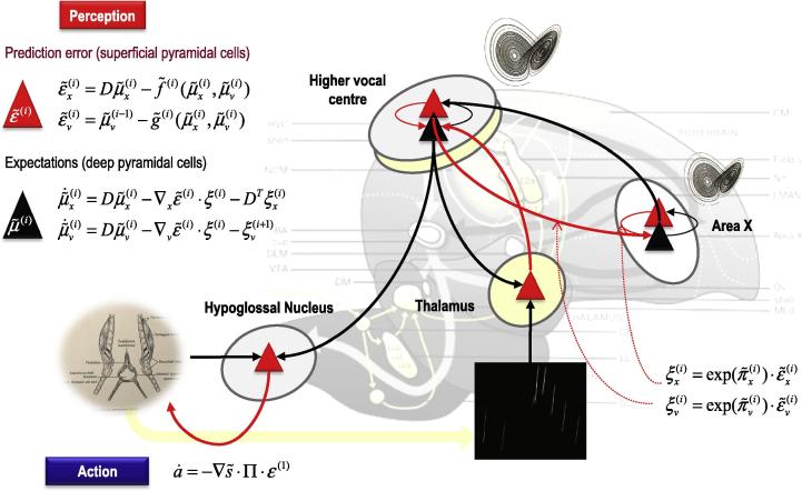
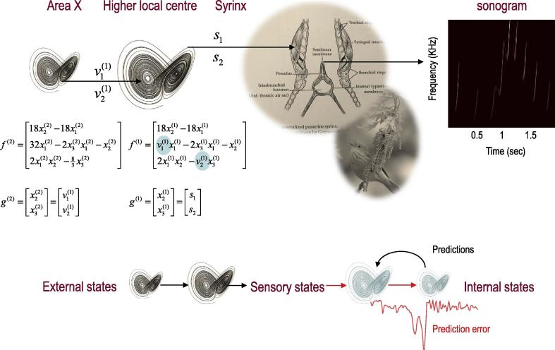
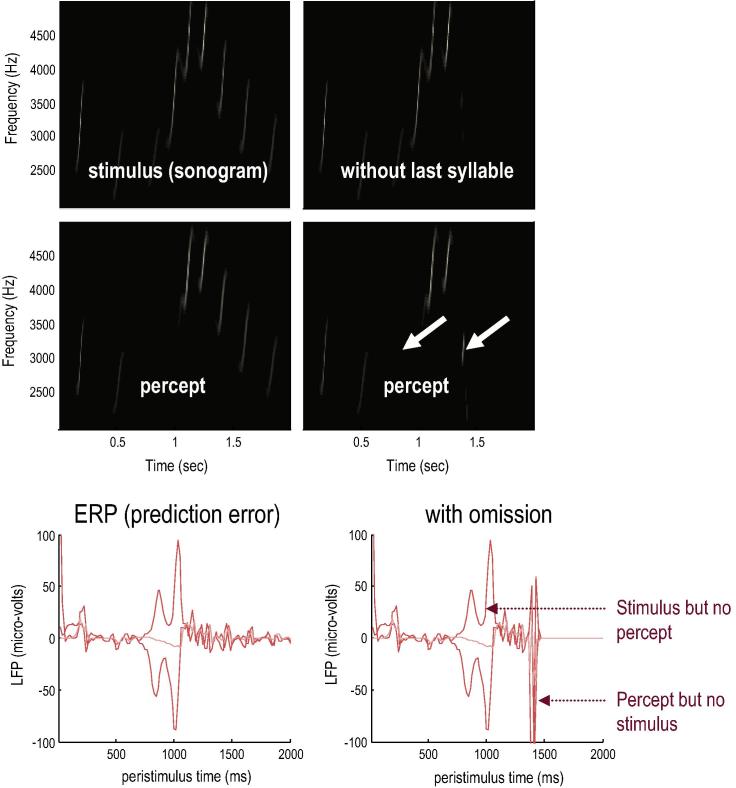
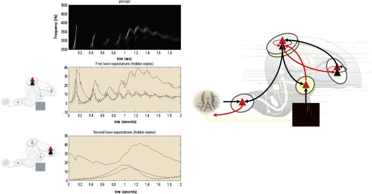
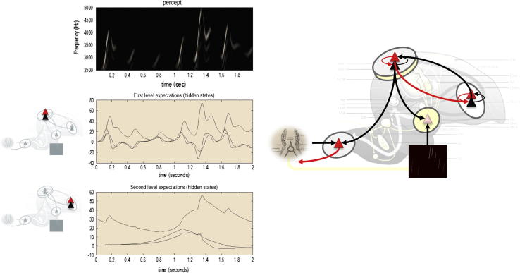
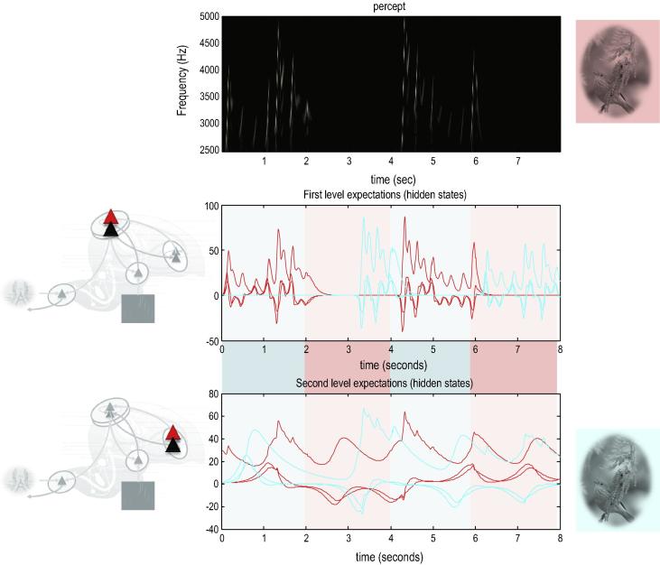
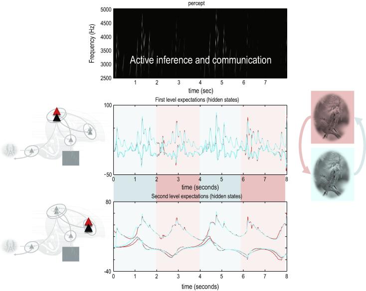
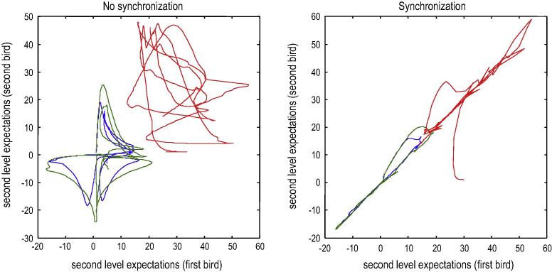
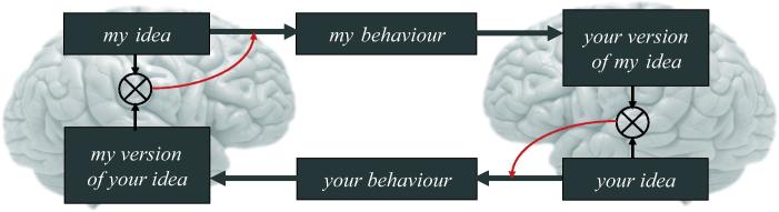
This paper considers communication in terms of inference about the behaviour of others (and our own behaviour). It is based on the premise that our sensations are largely generated by other agents like ourselves. This means, we are trying to infer how our sensations are caused by others, while they are trying to infer our behaviour: for example, in the dialogue between two speakers. We suggest that the infinite regress induced by modelling another agent - who is modelling you - can be finessed if you both possess the same model. In other words, the sensations caused by others and oneself are generated by the same process. This leads to a view of communication based upon a narrative that is shared by agents who are exchanging sensory signals. Crucially, this narrative transcends agency - and simply involves intermittently attending to and attenuating sensory input. Attending to sensations enables the shared narrative to predict the sensations generated by another (i.e. to listen), while attenuating sensory input enables one to articulate the narrative (i.e. to speak). This produces a reciprocal exchange of sensory signals that, formally, induces a generalised synchrony between internal (neuronal) brain states generating predictions in both agents. We develop the arguments behind this perspective, using an active (Bayesian) inference framework and offer some simulations (of birdsong) as proof of principle.
Overview
The claims and statistics of this paper haven’t been checked yet.
Run the check — free, no account needed. It reads the open-access text and checks the sources it cites.
Integrity signals
Registry
Cites
Statistics
Figures
Verification
Claims the paper makes
The claims and statistics of this paper haven’t been checked yet.
Run the check — free, no account needed. It reads the open-access text and checks the sources it cites.
Claims other papers make about this one
Each is checked against this paper’s own text: does it say what the citing paper says it does?
The source backs part of the claim, not all of it — or backs it for a different population, condition or comparison.
In the citing paper
“This brings with it an extra inference problem; namely, the attribution of agency. In other words, if we use the same models to explain our own behavior and the observed consequences of another’s behavior, then we also have to carefully infer agency (in order to appropriately attenuate proprioceptive precision and preclude echopraxia, Friston and Frith, 2015).”
From 'Seeing the Dark': Grounding Phenomenal Transparency and Opacity in Precision Estimation for Active Inference (2018) · cites this paper as Friston and Frith, 2015
Experimental — accuracy not yet measured
Self-check
Percentages, sums and reported differences re-computed from the paper’s own numbers.
The self-check needs the paper’s full text.
Citations
Cites
Whatever next? Predictive brains, situated agents, and the future of cognitive science
Clark, A. (2013) · Behavioral and Brain Sciences · doi:10.1017/s0140525x12000477 · Cited by 5,924
Rao, R. P. N., & Ballard, D. H. (1999) · Nature Neuroscience · doi:10.1038/4580 · Cited by 5,483
The weak coherence account: detail-focused cognitive style in autism spectrum disorders
Happé, F., & Frith, U. (2006) · Journal of Autism and Developmental Disorders · doi:10.1007/s10803-005-0039-0 · Cited by 2,884
Canonical Microcircuits for Predictive Coding
Bastos, A. M., Usrey, W. M., Adams, R. A., Mangun, G. R., Fries, P., & Friston, K. J. (2012) · Neuron · doi:10.1016/j.neuron.2012.10.038 · Cited by 2,421 · cited 1×
“In a companion paper (Friston & Frith, 2015), we demonstrate how communication facilitates long-term changes in generative models that are trying to predict each other.”
BackgroundSelf-citationHohwy, J. (2013) · doi:10.1093/acprof:oso/9780199682737.001.0001 · Cited by 1,914
Foundations of Language: Brain, Meaning, Grammar, Evolution
Jackendoff, R. S. (2002) · Cited by 1,858
Interoceptive inference, emotion, and the embodied self
Seth, A. K. (2013) · Trends in Cognitive Sciences · doi:10.1016/j.tics.2013.09.007 · Cited by 1,816 · cited 1×
“A particularly interesting issue here is interoceptive inference (Seth, 2013), and how visual cues about the emotional states of others can be interpreted in relation to generative models of our own interoceptive cues: see (Kanaya, Matsushima, & Yokosawa, 2012).”
BackgroundPredictive coding under the free-energy principle
Friston, K., & Kiebel, S. (2009) · Philosophical Transactions of the Royal Society B: Biological Sciences · doi:10.1098/rstb.2008.0300 · Cited by 1,579
Self-citationHierarchical Bayesian inference in the visual cortex
Lee, T. S., & Mumford, D. (2003) · Journal of the Optical Society of America A · doi:10.1364/josaa.20.001434 · Cited by 1,473 · cited 3×
“…been formalised in recent decades to cover deep or hierarchical Bayesian inference – about the causes of our sensations – and how these inferences induce beliefs, movement and behaviour (Clark, 2013b; Dayan, Hinton, & Neal, 1995; Friston, Kilner, & Harrison, 2006; Hohwy, 2013; Lee & Mumford, 2003).”
BackgroundPerceiving is believing: a Bayesian approach to explaining the positive symptoms of schizophrenia
Fletcher, P. C., & Frith, C. D. (2009) · Nature Reviews Neuroscience · doi:10.1038/nrn2536 · Cited by 1,462
Self-citation
Research works printed but not linked: 1
- Clark, 2013, The many faces of precision, Frontiers in Psychology, 4, 270
Cited by
Sorted by citations
Items 301–361 of 361
THE UNDERLYING BIOMECHANICS OF OUR BRAIN
Young, J. H. (2023) · Wiley eBooks · doi:10.1002/9781119767398.ch1
MINDING THE PORTFOLIO OF BELIEFS II
Young, J. H. (2023) · Wiley eBooks · doi:10.1002/9781119767398.ch10
Young, J. H. (2023) · Wiley eBooks · doi:10.1002/9781119767398.ch6
INTRODUCTION TO THE MBSAT PROGRAM: ESSENTIAL FOUNDATIONS TO MAKE YOUR MBSAT TRAINING EFFECTIVE
Young, J. H. (2023) · Wiley eBooks · doi:10.1002/9781119767398.ch4
MINDING BETA IV ‐ ACTION IMPULSES
Young, J. H. (2023) · Wiley eBooks · doi:10.1002/9781119767398.ch8
Young, J. H. (2023) · Wiley eBooks · doi:10.1002/9781119767398.ch7
Young, J. H. (2023) · Wiley eBooks · doi:10.1002/9781119767398.ref
MINDING THE PORTFOLIO OF BELIEFS III
Young, J. H. (2023) · Wiley eBooks · doi:10.1002/9781119767398.ch11
THE MBSAT PROGRAM AND ITS DISTINCTIVE FEATURES
Young, J. H. (2023) · Wiley eBooks · doi:10.1002/9781119767398.ch3
FREE ENERGY, ACTIVE INFERENCE AND THE PREDICTIVE BETA MIND IN MBSAT
Young, J. H. (2023) · Wiley eBooks · doi:10.1002/9781119767398.ch2
Friston, K. J. (2023) · Physics of Life Reviews · doi:10.1016/j.plrev.2023.06.007
Self-citationL. S. Vygotsky: Journey to the West
Mikhailov, I. F. (2023) · Philosophical Letters Russian and European Dialogue · doi:10.17323/2658-5413-2023-6-3-187-205
Eluchans, M., Donnarumma, F., & Pezzulo, G. (2023) · Physics of Life Reviews · doi:10.1016/j.plrev.2023.12.009
Sadato, N. (2024) · Rinsho Shinkeigaku · doi:10.5692/clinicalneurol.cn-001944
Brain and world—converging free energy principle and dynamic layer model of brain
Northoff, G. (2024) · Elsevier eBooks · doi:10.1016/b978-0-12-821935-5.00037-5
Measure for Measure: Operationalising Cognitive Realism
Beni, M. D. (2024) · Minds and Machines · doi:10.1007/s11023-024-09690-0
Gambi, C., Zhang, F., & Pickering, M. J. (2024) · Journal of Neurolinguistics · doi:10.1016/j.jneuroling.2024.101229
Social behavior in primates and its neural correlates
Qi, G., & Chang, S. W. C. (2025) · Elsevier eBooks · doi:10.1016/b978-0-443-27380-3.00002-6
Cultural bodybuilding: The embodied influence of culture on perception and action
Albarracin, M. (2025) · The Psychology of learning and motivation/The psychology of learning and motivation · doi:10.1016/bs.plm.2025.02.002 · Cited by 1
The Future of Perceptual Dysregulation in Psychiatric Nosology
Powers, A. R., & Khalsa, S. S. (2025) · Current topics in behavioral neurosciences · doi:10.1007/7854_2025_596
Scenes from a Marriage: How We Found Our Way from Experimental Psychology to Social Neuroscience
Frith, U., & Frith, C. (2025) · Annual Review of Psychology · doi:10.1146/annurev-psych-012425-033822
Self-citationBrains, Bodies, and Their Worlds: Towards a Model of Predictive Social Actors
Cheadle, J. E., Davidson-Turner, K., & Goosby, B. J. (2025) · Handbooks of sociology and social research · doi:10.1007/978-3-031-95615-7_16
Neural and behavioral dynamics of dyadic rhythm coordination across limb pairings
Han, H., Zhao, Z., Lin, L., Li, C., & Jin, X. (2025) · Behavioural Brain Research · doi:10.1016/j.bbr.2025.115877 · Cited by 1
De Felice, S., Hatilova, A., Trojan, F., Tsui, I., & Hamilton, A. F. D. C. (2024) · Figshare · doi:10.6084/m9.figshare.26615401
Active Inference Modeling of Socially Shared Cognition in Virtual Reality
Arima, Y., & Okada, M. (2026) · Sensors · doi:10.3390/s26020604
Against (theory-neutral) method (in consciousness science)
Beni, M. D. (2026) · Neuroscience of Consciousness · doi:10.1093/nc/niag003 · Cited by 2
Covert neural and autonomic signatures of shared perception
Yavuz, M., Esmaily, J., Bahrami, B., & Deroy, O. D. (2026) · Social Cognitive and Affective Neuroscience · doi:10.1093/scan/nsag009
Béres, L., Nagy, P., Pólya, T., Weiss, B., Boncz, A., & Winkler, I. (2026) · Frontiers in Psychology · doi:10.3389/fpsyg.2026.1655164
Freud’s Model of the Mind Within a Predictive Processing Neuroscientific Paradigm
Stänicke, E., Hovet, B. S., & Stänicke, L. I. (2026) · Entropy · doi:10.3390/e28030318
Epistemic Drift in Mind-Model Systems
Søgaard, A., Rajcic, N., & Scott, A. E. (2026) · Minds and Machines · doi:10.1007/s11023-026-09772-1
Embodied predictive processing: A unifying generative principle for cognitive development
Nagai, Y. (2026) · Advances in child development and behavior · doi:10.1016/bs.acdb.2026.04.002
Rhythm in Speech and Language Disabilities
Meyer, L., & Strauß, A. (2026) · Cambridge University Press eBooks · doi:10.1017/9781009295888.049
Ziegler, W., & Aichert, I. (2026) · Cambridge University Press eBooks · doi:10.1017/9781009295888.052
Roos, M., Storm, H., Zimmer, L., & Schuwerk, T. (2026) · Autism · doi:10.1177/13623613261443728
Miyano, S., & SHIONO, T. (2026) · Entropy · doi:10.3390/e28050491
Ellis, G. (2026) · Oxford University Press eBooks · doi:10.1093/9780198950189.005.0001
The influence of task demands on joint action planning
Friebe, K., Sebanz, N., & Knoblich, G. (2026) · Acta Psychologica · doi:10.1016/j.actpsy.2026.107057
Computational spirits: a neuroscientific account of psychedelic entity encounters
Mago, J., Deane, G., Sandved-Smith, L., Safron, A., Timmermann, C., Ramstead, M. J. D., Dupuis, D., Carhart-Harris, R. L., Greenway, K. T., & Lifshitz, M. (2026) · Neuroscience of Consciousness · doi:10.1093/nc/niaf069
Larson, D. O., Sarto‐Jackson, I., & Fischer, B. (2026) · Biological Theory · doi:10.1007/s13752-026-00536-9
Parvizi-Wayne, D., Pedersen, R., & Rankin, J. (2026) · Review of Philosophy and Psychology · doi:10.1007/s13164-026-00828-w
Yamashita, Y. (2026) · Journal of the Robotics Society of Japan · doi:10.7210/jrsj.44.480
Interpersonal neural coordination tracks interaction quality during naturalistic conversation
Domínguez-Arriola, M. E., Lam, P. C. H., Pérez, A., & Pell, M. D. (2026) · NeuroImage · doi:10.1016/j.neuroimage.2026.122090 · Cited by 1
Differentiation of cortical areas: effects of free energy minimization with broken symmetry
Wright, J. J., & Bourke, P. D. (2026) · Cerebral Cortex · doi:10.1093/cercor/bhag068
Valenzuela, L., Cavallaro, R., Mangeng, A., Pérez-Arenas, X., Carollo, A., Esposito, G., Medel, V., & Soto, V. (2026) · NeuroImage · doi:10.1016/j.neuroimage.2026.122116
Acting under uncertainty: Prediction, contingency, and the function of magic
Sørensen, J. (2026) · Evolution and Human Behavior · doi:10.1016/j.evolhumbehav.2026.106941
Hierarchical processing of continuous natural language: From monologue to conversation
Wang, M., & Lu, C. (2026) · Brain and Language · doi:10.1016/j.bandl.2026.105815
Embodied intersubjectivity in motion: Neurodynamics of kinesthetic empathy in psychotherapy
Vaisvaser, S. (2026) · The Arts in Psychotherapy · doi:10.1016/j.aip.2026.102513
Проективное контейнирование как компенсация интероцепции: Единая нейрофизиологическая модельPreprint
Bikbulatov, D. (2026) · doi:10.24108/preprints-3115931
EMI-EDU: reframing learning and education through energy, mass and information
Firaux, T., Damiani, P., & Cavaglià, M. (2026) · Frontiers in Human Neuroscience · doi:10.3389/fnhum.2026.1761644
Beasley, D. (2026) · Frontiers in Psychiatry · doi:10.3389/fpsyt.2026.1886942
Newell, D., Segal, S., Rossettini, G., O’Neill, S. F. D., Lothe-Raven, T., Lothe, L. R., Weiniger, S., du Rose, A., Beira, B., Walker, K., et al. (2026) · Chiropractic & Manual Therapies · doi:10.1186/s12998-026-00669-5
Altered integration of bodily and visual signals in visual snow syndrome
Beukelaer, S. D., Schloßmacher, I., Aeschlimann, S. A., Klein, A., Szukics, A., Ertl, M., & Schankin, C. J. (2026) · Cephalalgia · doi:10.1177/03331024261480300
Predictions and goals modulate use of partner's gaze during joint action with humanoid robots
Pérez-Osorio, J., Wiese, E., Abubshait, A., & Wykowska, A. (2026) · Acta Psychologica · doi:10.1016/j.actpsy.2026.107838
Exceptional cognition and the limits of social prediction
Wang, P., Xia, Y., Tang, X., Vincent, J., Zou, L., Law, E. L., Hertwig, R., & Paas, F. (2026) · Trends Open · doi:10.1016/j.treopn.2026.08.020
Teoharie, C. (2026) · Frontiers in Psychology · doi:10.3389/fpsyg.2026.1860291
Bai, Y., & Zhang, Q. (2026) · Brain Research · doi:10.1016/j.brainres.2026.150594
Reframing the lived experience of persistent dizziness: insights from active inference
Broberg, M. A., Thacker, M., Friston, K. J., & Esteves, J. E. (2026) · Frontiers in Psychology · doi:10.3389/fpsyg.2026.1867836
Self-citationLucchiari, C., & Vanutelli, M. E. (2026) · Brain Sciences · doi:10.3390/brainsci16101104
Theory of mind and mentalizing
Votinov, M. (2026) · Elsevier eBooks · doi:10.1016/b978-0-443-34080-2.00015-9
Social Reality Construction via Active Inference: Modeling the Dialectic of Conformity and Creativity
Nomura, K., & Horii, T. (2026) · arXiv
“Communication under active inference has further been shown to drive generalized synchrony and long-term convergence of generative models between agents (Friston and Frith, 2015a,b).”
A free energy principle for a particular physics
Friston, K. (2019) · arXiv · doi:10.48550/arxiv.1906.10184 · Cited by 222
Self-citation
Metadata
- Authors
- Friston, K., & Frith, C.
- Affiliations
- Wellcome Centre for Human Neuroimaging (GB)
- Corresponding author
- Friston, Karl
- ORCID
- Friston, Karl
- Venue
- Consciousness and Cognition
- Publisher
- Elsevier BV
- Published
- 2015-11
- Volume
- 36
- Pages
- 390-405
- ISSN
- 1053-8100 (ISSN-L)
- PMC
- PMC4553904
- OpenAlex
- W2024149692
- Cited by
- 359
- References
- 82
- Citations by year
- 2026: 44 · 2025: 31 · 2024: 33 · 2023: 43 · 2022: 41 · 2021: 41 · 2020: 21 · 2019: 22 · 2018: 30 · 2017: 26 · 2016: 22 · 2015: 5
- FWCI
- 16.63
- Type
- journal article
- Language
- en
- Open access
- hybrid
- doi.org
- Locations
- Consciousness and Cognition (publishedVersion, cc-by)
- PubMed Central (publishedVersion, cc-by)
- PubMed (publishedVersion)
- UCL Discovery (University College London) (submittedVersion)
- Funders
- Wellcome Trust (091593, 088130)
- Topics
- Life Sciences › Neuroscience › Cognitive Neuroscience › Embodied and Extended Cognition
- Social Sciences › Psychology › Social Psychology › Action Observation and Synchronization
- Social Sciences › Psychology › Developmental and Educational Psychology › Child and Animal Learning Development
- Keywords
- communication, joint action, shared narratives, Bayesian inference, infinite regress, shared models, sensory prediction, attention, attenuation, bird song, social cognition
- MeSH terms
- Animals, Attention, Communication, Humans, Models, Theoretical, Perception, Sensation, Thinking, Theory of Mind
About these checks
Registry, retraction, Cites and statistics results are computed, not judged, with one exception: a printed reference that no index lists is read once by a model before it counts as a citation error. Claims are extracted by a model and kept only when their quote appears verbatim in the text; each cited source is then checked, with a model’s help, for whether it says what the claim relies on. Those verdicts can be wrong — read the claim’s quote and the cited source before relying on one.
Statistics and arithmetic are recomputed, not judged.
Confidence bands are shown only for fields calibrated on our annotated test set. None is calibrated yet, so no band is shown.
What counts as a claim ›How we measure confidence ›How we check this ›
Are you an author, or do you see a problem with this page? Request a review
