

The DOI matches its Crossref record; 59 of the 59 references it cites were found in a registry or an index.
Climate Forcing and Trends of Organic Aerosols in the Community Earth System Model (CESM2)
Open accessAbstract
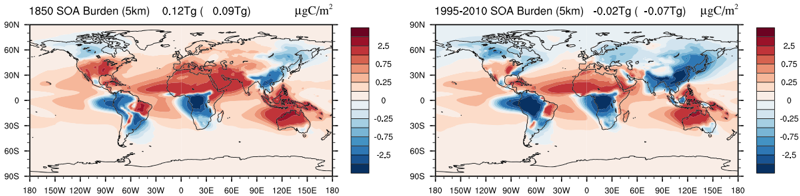
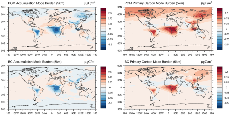
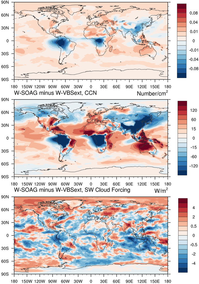
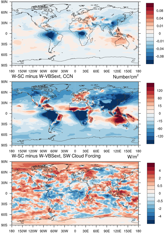
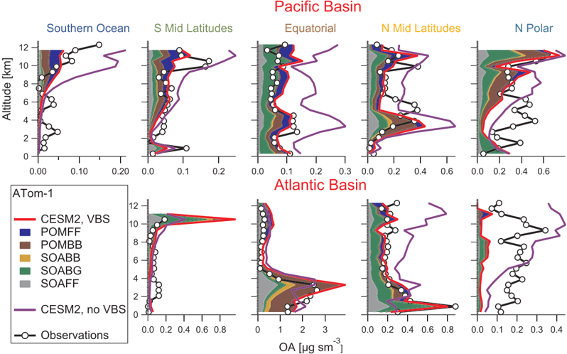
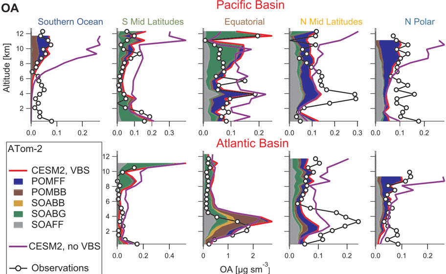
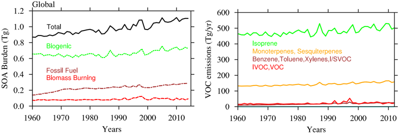
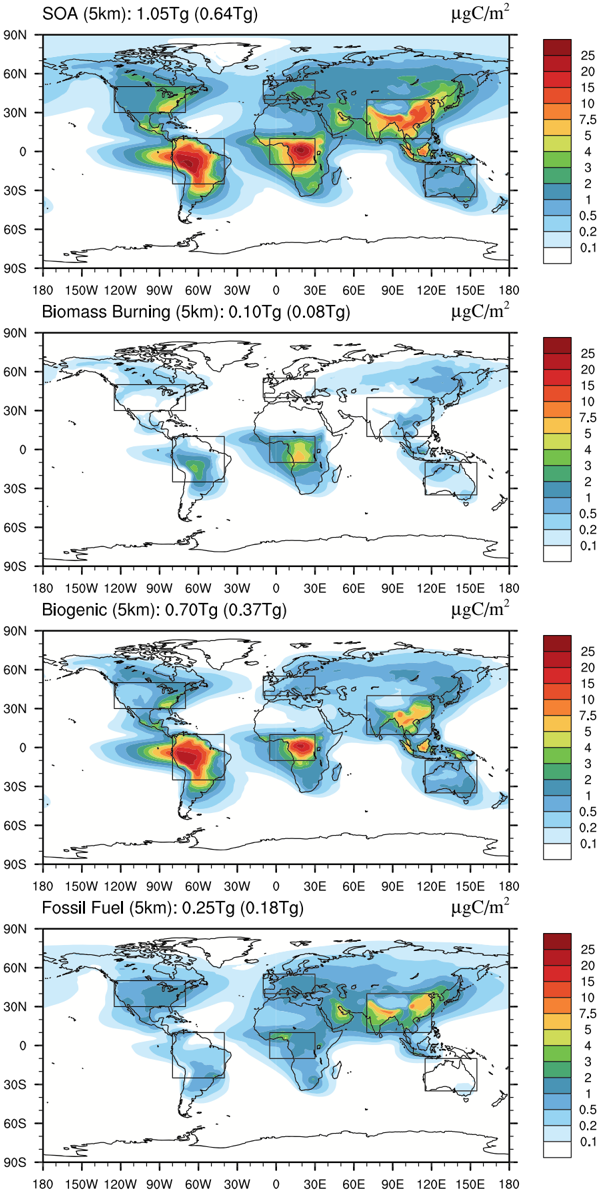
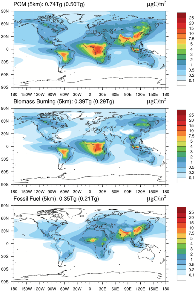
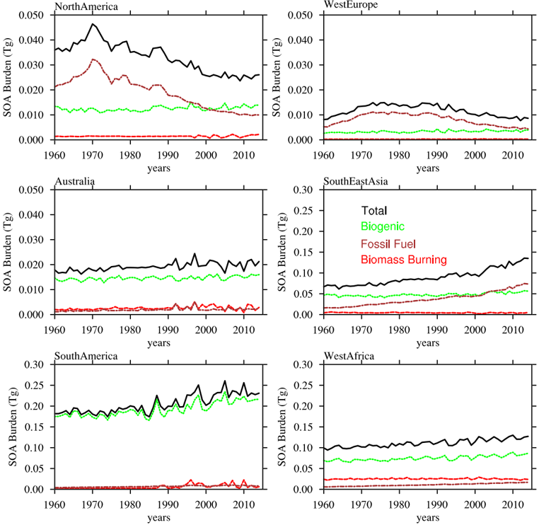
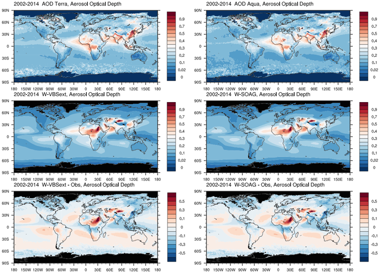
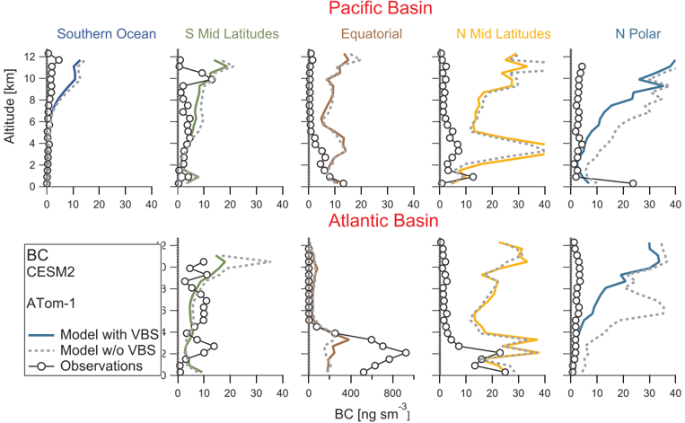
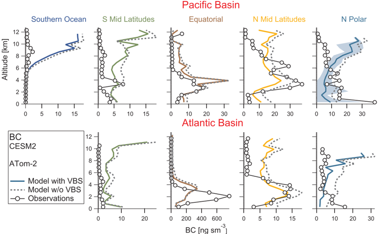
The Community Earth System Model version 2 (CESM2) includes three main atmospheric configurations: the Community Atmosphere Model version 6 (CAM6) with simplified chemistry and a simplified organic aerosol (OA) scheme, CAM6 with comprehensive tropospheric and stratospheric chemistry representation (CAM6‐chem), and the Whole Atmosphere Community Climate Model version 6 (WACCM6). Both, CAM6‐chem and WACCM6 include a more comprehensive secondary organic aerosols (SOA) approach using the Volatility Basis Set (VBS) scheme and prognostic stratospheric aerosols. This paper describes the different OA schemes available in the different atmospheric configurations of CESM2 and discusses differences in aerosol burden and resulting climate forcings. Derived OA burden and trends differ due to differences in OA formation using the different approaches. Regional differences in Aerosol Optical Depth with larger values using the comprehensive approach occur over SOA source regions. Stronger increasing SOA trends between 1960 and 2015 in WACCM6 compared to CAM6 are due to increasing biogenic emissions aligned with increasing surface temperatures. Using the comprehensive SOA approach further leads to improved comparisons to aircraft observations and SOA formation of ≈143 Tg/yr. We further use WACCM6 to identify source contributions of OA from biogenic, fossil fuel, and biomass burning emissions, to quantify SOA amounts and trends from these sources. Increasing SOA trends between 1960 and 2015 are the result of increasing biogenic emissions aligned with increasing surface temperatures. Biogenic emissions are at least two thirds of the total SOA burden. In addition, SOA source contributions from fossil fuel emissions become more important, with largest values over Southeast Asia. The estimated total anthropogenic forcing of OA in WACCM6 for 1995–2010 conditions is −0.43 W/m 2, mostly from the aerosol direct effect.
Overview
The claims and statistics of this paper haven’t been checked yet.
Run the check — free, no account needed. It reads the open-access text and checks the sources it cites.
Integrity signals
Registry
Cites
Statistics
Figures

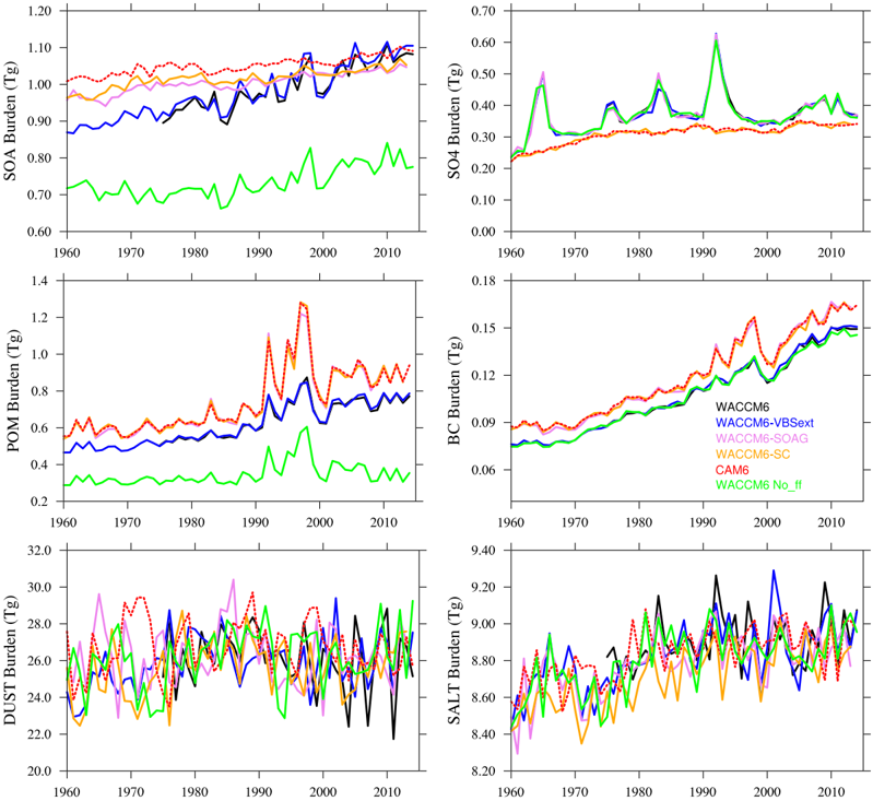

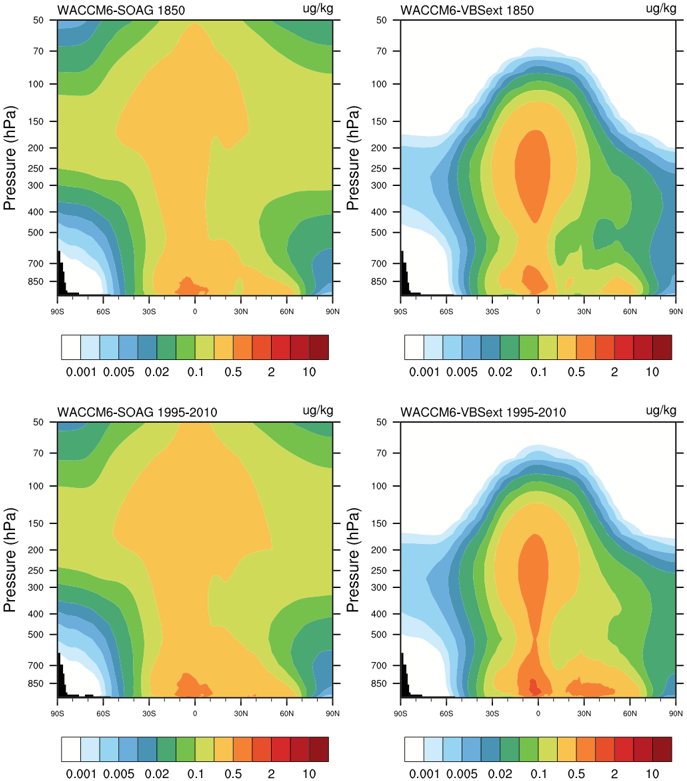

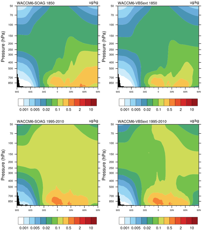
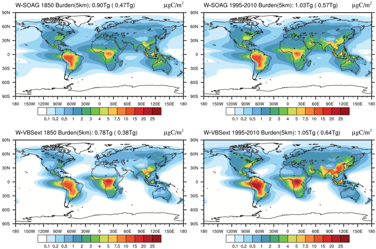





Verification
Claims the paper makes
The claims and statistics of this paper haven’t been checked yet.
Run the check — free, no account needed. It reads the open-access text and checks the sources it cites.
Claims other papers make about this one
Each is checked against this paper’s own text: does it say what the citing paper says it does?
In the citing paper
“CESM2(WACCM6) has been evaluated against earlier model versions and observations - including NASA ATom aircraft profiles (Tilmes et al., 2019), Tropospheric Ozone Assessment Report (TOAR) surface ozone data (Emmons et al., 2020), and Measurements of Pollution in The Troposphere (MOPITT) carbon monoxide observations (Schwantes et al., 2020) - showing good agreement with ozonesonde data and season”
From Air quality impacts of stratospheric aerosol injections are likely small and mainly driven by changes in climate, not aerosol settling (2026) · cites this paper as Tilmes et al., 2019
In the citing paper
“These limitations notwithstanding, the interactive chemistry-climate framework of WACCM allows us to capture coupled meteorological, chemical, and radiative feedbacks that are central to evaluating the air quality response to stratospheric aerosol injection (Tilmes et al., 2019).”
From Air quality impacts of stratospheric aerosol injections are likely small and mainly driven by changes in climate, not aerosol settling (2026) · cites this paper as Tilmes et al., 2019
Self-check
Percentages, sums and reported differences re-computed from the paper’s own numbers.
The self-check needs the paper’s full text.
Citations
Cites
Guenther, A., Jiang, X., Heald, C. L., Sakulyanontvittaya, T., Duhl, T. R., Emmons, L. K., & Wang, X. (2012) · Geoscientific model development · doi:10.5194/gmd-5-1471-2012 · Cited by 4,126
Self-citationThe formation, properties and impact of secondary organic aerosol: current and emerging issues
Hallquist, M., Wenger, J., Baltensperger, U., Rudich, Y., Simpson, D. M., Claeys, M., Dommen, J., Donahue, N. M., George, C., Goldstein, A. H., et al. (2009) · Atmospheric chemistry and physics · doi:10.5194/acp-9-5155-2009 · Cited by 4,039
Self-citationThe Collection 6 MODIS aerosol products over land and ocean
Levy, R. C., Mattoo, S., Munchak, L. A., Remer, L. A., Sayer, A. M., Patadia, F., & Hsu, N.-Y. C. (2013) · Atmospheric measurement techniques · doi:10.5194/amt-6-2989-2013 · Cited by 2,327
Hoesly, R. M., Smith, S. J., Feng, L., Klimont, Z., Janssens-Maenhout, G., Pitkanen, T., Seibert, J. J., Vu, L., Andres, R. J., Bolt, R. M., et al. (2018) · Geoscientific Model Development · doi:10.5194/gmd-11-369-2018 · Cited by 2,203
Field-Deployable, High-Resolution, Time-of-Flight Aerosol Mass Spectrometer
DeCarlo, P. F., Kimmel, J. R., Trimborn, A., Northway, M. J., Jayne, J. T., Aiken, A. C., Gonin, M., Führer, K., Horvath, T. D., Docherty, K. S., et al. (2006) · Analytical Chemistry · doi:10.1021/ac061249n · Cited by 2,151
Self-citationCanagaratna, M. R., Jayne, J. T., Jimenez, J. L., Allan, J. D., Alfarra, M. R., Zhang, Q., Onasch, T. B., Drewnick, F., Coe, H., Middlebrook, A. M., et al. (2007) · Mass Spectrometry Reviews · doi:10.1002/mas.20115 · Cited by 1,953
Self-citationRethinking Organic Aerosols: Semivolatile Emissions and Photochemical Aging
Robinson, A. L., Donahue, N. M., Shrivastava, M. K., Weitkamp, E. A., Sage, A. M., Grieshop, A. P., Lane, T. E., Pierce, J. R., & Pandis, S. Ν. (2007) · Science · doi:10.1126/science.1133061 · Cited by 1,945
Self-citationWiedinmyer, C., Akagi, S. K., Yokelson, R. J., Emmons, L. K., Al-Saadi, J. A., Orlando, J. J., & Soja, A. J. (2011) · Geoscientific Model Development · doi:10.5194/gmd-4-625-2011 · Cited by 1,850
Self-citationChin, M., Ginoux, P. A., Kinne, S., Torres, O., HOLBEN, B. N., Duncan, B. N., Martin, R. V., Logan, J. A., Higurashi, A., & Nakajima, T. (2002) · Journal of the Atmospheric Sciences · doi:10.1175/1520-0469(2002)059 · Cited by 1,580
Gas/Particle Partitioning and Secondary Organic Aerosol Yields
Odum, J. R., Hoffmann, T., Bowman, F., Collins, D. R., Flagan, R. C., & Seinfeld, J. H. (1996) · Environmental Science & Technology · doi:10.1021/es950943+ · Cited by 1,530
Cited by
Sorted by citations
The Community Earth System Model Version 2 (CESM2)
Danabasoglu, G., Lamarque, J., Bacmeister, J. T., Bailey, D. A., DuVivier, A. K., Edwards, J., Emmons, L. K., Fasullo, J., García, R. R., Gettelman, A., et al. (2020) · Journal of Advances in Modeling Earth Systems · doi:10.1029/2019ms001916 · Cited by 3,408
Self-citation(IPCC), I. P. O. C. C. (2023) · Cambridge University Press eBooks · doi:10.1017/9781009157896.008 · Cited by 756
The Chemistry Mechanism in the Community Earth System Model Version 2 (CESM2)
Emmons, L. K., Schwantes, R. H., Orlando, J. J., Tyndall, G., Kinnison, D., Lamarque, J., Marsh, D., Mills, M. J., Tilmes, S., Bardeen, C., et al. (2020) · Journal of Advances in Modeling Earth Systems · doi:10.1029/2019ms001882 · Cited by 613
Self-citationHistorical and future changes in air pollutants from CMIP6 models
Turnock, S. T., Allen, R. J., Andrews, M. B., Bauer, S. E., Deushi, M., Emmons, L. K., Good, P., Horowitz, L. W., John, J. G., Michou, M., et al. (2020) · Atmospheric chemistry and physics · doi:10.5194/acp-20-14547-2020 · Cited by 369
Self-citationTropospheric ozone in CMIP6 simulations
Griffiths, P. T., Murray, L. T., Zeng, G., Shin, Y. M., Abraham, N. L., Archibald, A. T., Deushi, M., Emmons, L. K., Galbally, I. E., Hassler, B., et al. (2021) · Atmospheric Chemistry and Physics · doi:10.5194/acp-21-4187-2021 · Cited by 289
Self-citationSecondary organic aerosol formed by condensing anthropogenic vapours over China’s megacities
Nie, W., Yan, C., Huang, D. D., Wang, Z., Liu, Y., Qiao, X., Guo, Y., Tian, L., Zheng, P., Xu, Z., et al. (2022) · Nature Geoscience · doi:10.1038/s41561-022-00922-5 · Cited by 215
Effective radiative forcing from emissions of reactive gases and aerosols – a multi-model comparison
Thornhill, G. D., Collins, W. J., Kramer, R. J., Olivié, D., Skeie, R. B., O’Connor, F. M., Abraham, N. L., Checa‐Garcia, R., Bauer, S. E., Deushi, M., et al. (2021) · Atmospheric chemistry and physics · doi:10.5194/acp-21-853-2021 · Cited by 203
Self-citationGlobal Changes in Secondary Atmospheric Pollutants During the 2020 COVID‐19 Pandemic
Gaubert, B., Bouarar, I., Doumbia, T., Liu, Y., Stavrakou, T., Deroubaix, A. M., Darras, S., Elguindi, N., Granier, C., Lacey, F. G., et al. (2021) · Journal of Geophysical Research Atmospheres · doi:10.1029/2020jd034213 · Cited by 144
Self-citationExploring dimethyl sulfide (DMS) oxidation and implications for global aerosol radiative forcing
Fung, K. M., Heald, C. L., Kroll, J. H., Wang, S., Jo, D. S., Gettelman, A., Lu, Z., Liu, X., Zaveri, R. A., Apel, E. C., et al. (2022) · Atmospheric chemistry and physics · doi:10.5194/acp-22-1549-2022 · Cited by 152
Self-citationHodžić, A., Campuzano‐Jost, P., Bian, H., Chin, M., Colarco, P. R., Day, D. A., Froyd, K. D., Heinold, B., Jo, D. S., Katich, J. M., et al. (2020) · Atmospheric chemistry and physics · doi:10.5194/acp-20-4607-2020 · Cited by 144
Self-citationTilmes, S., MacMartin, D. G., Lenaerts, J. T. M., van Kampenhout, L., Muntjewerf, L., Xia, L., Harrison, C. S., Krumhardt, K. M., Mills, M. J., Kravitz, B., et al. (2020) · Earth System Dynamics · doi:10.5194/esd-11-579-2020 · Cited by 146
Self-citationMulti-model intercomparisons of air quality simulations for the KORUS-AQ campaign
Park, R. J., Oak, Y. J., Emmons, L. K., Kim, C., Pfister, G. G., Carmichael, G. R., Saide, P. E., Cho, S.-Y., Kim, S., Woo, J., et al. (2021) · Elementa Science of the Anthropocene · doi:10.1525/elementa.2021.00139 · Cited by 129
Self-citationCorrecting model biases of CO in East Asia: impact on oxidant distributions during KORUS-AQ
Gaubert, B., Emmons, L. K., Raeder, K., Tilmes, S., Miyazaki, K., Arellano, A. F., Elguindi, N., Granier, C., Tang, W., Barré, J., et al. (2020) · Atmospheric chemistry and physics · doi:10.5194/acp-20-14617-2020 · Cited by 134
Self-citationSchwantes, R. H., Emmons, L. K., Orlando, J. J., Barth, M. C., Tyndall, G. S., Hall, S. R., Ullmann, K., St. Clair, J. M., Blake, D. R., Wisthaler, A., et al. (2020) · Atmospheric Chemistry and Physics · doi:10.5194/acp-20-3739-2020 · Cited by 112
Self-citationMortier, A., Gliß, J., Schulz, M., Aas, W., Andrews, E. J., Bian, H., Chin, M., Ginoux, P. A., Hand, J. L., HOLBEN, B. N., et al. (2020) · Atmospheric chemistry and physics · doi:10.5194/acp-20-13355-2020 · Cited by 106
Self-citationSpurious Late Historical‐Era Warming in CESM2 Driven by Prescribed Biomass Burning Emissions
Fasullo, J., Lamarque, J., Hannay, C., Rosenbloom, N. A., Tilmes, S., DeRepentigny, P., Jahn, A., & Deser, C. (2022) · Geophysical Research Letters · doi:10.1029/2021gl097420 · Cited by 105
Self-citationOne-third of global population at cancer risk due to elevated volatile organic compounds levels
Ying, X., Du, K., & Huang, Y. (2024) · npj Climate and Atmospheric Science · doi:10.1038/s41612-024-00598-1 · Cited by 95
Tang, W., Emmons, L. K., Buchholz, R. R., Wiedinmyer, C., Schwantes, R. H., He, C., Kumar, R., Pfister, G. G., Worden, H. M., Hornbrook, R. S., et al. (2022) · Journal of Geophysical Research Atmospheres · doi:10.1029/2022jd036650 · Cited by 93
Self-citationDuVivier, A. K., Holland, M. M., Kay, J. E., Tilmes, S., Gettelman, A., & Bailey, D. A. (2020) · Journal of Geophysical Research Oceans · doi:10.1029/2019jc015934 · Cited by 88
Self-citationSchwantes, R. H., Lacey, F. G., Tilmes, S., Emmons, L. K., Lauritzen, P. H., Walters, S., Callaghan, P. F., Zarzycki, C. M., Barth, M. C., Jo, D. S., et al. (2022) · Journal of Advances in Modeling Earth Systems · doi:10.1029/2021ms002889 · Cited by 86
Self-citationA multiyear tropical Pacific cooling response to recent Australian wildfires in CESM2
Fasullo, J., Rosenbloom, N. A., & Buchholz, R. R. (2023) · Science Advances · doi:10.1126/sciadv.adg1213 · Cited by 75
Deng, Y., Inomata, S., Sato, K., Ramasamy, S., Morino, Y., Enami, S., & Tanimoto, H. (2021) · Atmospheric chemistry and physics · doi:10.5194/acp-21-5983-2021 · Cited by 70
Simpson, I. R., Rosenbloom, N. A., Danabasoglu, G., Deser, C., Yeager, S. G., McCluskey, C. S., Yamaguchi, R., Lamarque, J., Tilmes, S., Mills, M. J., et al. (2023) · Journal of Climate · doi:10.1175/jcli-d-22-0666.1 · Cited by 81
Self-citationArctic Sea Ice in Two Configurations of the CESM2 During the 20th and 21st Centuries
DeRepentigny, P., Jahn, A., Holland, M. M., & Smith, A. (2020) · Journal of Geophysical Research Oceans · doi:10.1029/2020jc016133 · Cited by 74
Ozone Anomalies in the Free Troposphere During the COVID‐19 Pandemic
Bouarar, I., Gaubert, B., Brasseur, G. P., Steinbrecht, W., Doumbia, T., Tilmes, S., Liu, Y., Stavrakou, T., Deroubaix, A. M., Darras, S., et al. (2021) · Geophysical Research Letters · doi:10.1029/2021gl094204 · Cited by 64
Self-citationClimate and air quality impacts due to mitigation of non-methane near-term climate forcers
Allen, R. J., Turnock, S. T., Nabat, P., Neubauer, D., Lohmann, U., Olivié, D., Oshima, N., Michou, M., Wu, T., Zhang, J., et al. (2020) · Atmospheric chemistry and physics · doi:10.5194/acp-20-9641-2020 · Cited by 67
Self-citationAtmospheric nanoparticle growth
Stolzenburg, D., Cai, R., Blichner, S. M., Kontkanen, J., Zhou, P., Makkonen, R., Kerminen, V., Kulmala, M., Riipinen, I., & Kangasluoma, J. (2023) · Reviews of Modern Physics · doi:10.1103/revmodphys.95.045002 · Cited by 68
Davis, N., Visioni, D., García, R. R., Kinnison, D. E., Marsh, D. R., Mills, M. J., Richter, J. H., Tilmes, S., Bardeen, C., Gettelman, A., et al. (2023) · Journal of Advances in Modeling Earth Systems · doi:10.1029/2022ms003579 · Cited by 73
Self-citationRamesh, K., Smith, A. K., García, R. R., Marsh, D. R., Sridharan, S., & Kumar, K. K. (2020) · Journal of Geophysical Research Atmospheres · doi:10.1029/2020jd033579 · Cited by 57
Global Anthropogenic Emissions of Full-Volatility Organic Compounds
Huang, L., Zhao, B., Wang, S., Chang, X., Klimont, Z., Huang, G., Zheng, H., & Hao, J. (2023) · Environmental Science & Technology · doi:10.1021/acs.est.3c04106 · Cited by 61
Zhang, W., Hai, S., Zhao, Y., Sheng, L., Zhou, Y., Wang, W., & Li, W. (2021) · Atmospheric Environment · doi:10.1016/j.atmosenv.2021.118393 · Cited by 53
Zaveri, R. A., Easter, R. C., Singh, B., Wang, H., Lu, Z., Tilmes, S., Emmons, L. K., Vitt, F. M., Zhang, R., Liu, X., et al. (2021) · Journal of Advances in Modeling Earth Systems · doi:10.1029/2020ms002346 · Cited by 53
Self-citationTang, W., Emmons, L. K., Wiedinmyer, C., Partha, D. B., Huang, Y., He, C., Zhang, J., Barsanti, K. C., Gaubert, B., Jo, D. S., et al. (2025) · Science Advances · doi:10.1126/sciadv.adr2616 · Cited by 57
Self-citationChemistry-driven changes strongly influence climate forcing from vegetation emissions
Weber, J., Archer‐Nicholls, S., Abraham, N. L., Shin, Y. M., Griffiths, P. T., Grosvenor, D. P., Scott, C. E., & Archibald, A. T. (2022) · Nature Communications · doi:10.1038/s41467-022-34944-9 · Cited by 54
Jo, D. S., Hodžić, A., Emmons, L. K., Tilmes, S., Schwantes, R. H., Mills, M. J., Campuzano‐Jost, P., Hu, W., Zaveri, R. A., Easter, R. C., et al. (2021) · Atmospheric chemistry and physics · doi:10.5194/acp-21-3395-2021 · Cited by 48
Self-citationFiore, A. M., Hancock, S. E., Lamarque, J., Correa, G. J. P., Chang, K., Ru, M., Cooper, O. R., Gaudel, A., Polvani, L. M., Sauvage, B., et al. (2022) · Environmental Research Climate · doi:10.1088/2752-5295/ac9cc2 · Cited by 54
Self-citationLou, S., Shrivastava, M., Easter, R. C., Yang, Y., Ma, P., Wang, H., Cubison, M. J., Campuzano‐Jost, P., Jimenez, J. L., Zhang, Q., et al. (2020) · Journal of Advances in Modeling Earth Systems · doi:10.1029/2020ms002266 · Cited by 47
Self-citationWhaley, C. H., Mahmood, R., von Salzen, K., Winter, B., Eckhardt, S., Arnold, S. R., Beagley, S. R., Becagli, S., Chien, R., Christensen, J. H., et al. (2022) · Atmospheric chemistry and physics · doi:10.5194/acp-22-5775-2022 · Cited by 47
Bhattarai, H., Tai, A. P. K., Martin, M. V., & Yung, D. H. Y. (2024) · The Science of The Total Environment · doi:10.1016/j.scitotenv.2024.174611 · Cited by 48
Jin, Q., Crippa, P., & Pryor, S. C. (2020) · Atmospheric Environment · doi:10.1016/j.atmosenv.2020.117718 · Cited by 41
Fasullo, J., Rosenbloom, N. A., Buchholz, R. R., Danabasoglu, G., Lawrence, D. M., & Lamarque, J. (2021) · Geophysical Research Letters · doi:10.1029/2021gl093841 · Cited by 41
Self-citationZhang, Y., Shindell, D. T., Seltzer, K. M., Shen, L., Lamarque, J., Zhang, Q., Zheng, B., Xing, J., Jiang, Z., & Zhang, L. (2021) · Atmospheric chemistry and physics · doi:10.5194/acp-21-16051-2021 · Cited by 42
Self-citationGao, C. Y., Heald, C. L., Katich, J. M., Luo, G., & Yu, F. (2022) · Journal of Geophysical Research Atmospheres · doi:10.1029/2022jd036524 · Cited by 37
Zhang, W., Li, W., An, X., Zhao, Y., Sheng, L., Hai, S., Li, X., Wang, F., Zi, Z., & Chu, M. (2022) · The Science of The Total Environment · doi:10.1016/j.scitotenv.2022.155231 · Cited by 36
Tilmes, S., Mills, M. J., Zhu, Y., Bardeen, C. G., Vitt, F., Yu, P., Fillmore, D., Liu, X., Toon, B., & Deshler, T. (2023) · Geoscientific Model Development · doi:10.5194/gmd-16-6087-2023 · Cited by 35
Self-citationWang, H., Lu, X., Seco, R., Stavrakou, T., Karl, T., Jiang, X., Gu, L., & Guenther, A. (2022) · Journal of Advances in Modeling Earth Systems · doi:10.1029/2022ms003174 · Cited by 38
A Multimodel Investigation of Asian Summer Monsoon UTLS Transport Over the Western Pacific
Pan, L. L., Kinnison, D. E., Liang, Q., Chin, M., Santee, M. L., Flemming, J., Smith, W. P., Honomichl, S., Bresch, J. F., Lait, L. R., et al. (2022) · Journal of Geophysical Research Atmospheres · doi:10.1029/2022jd037511 · Cited by 43
Self-citationHindley, N. P., Cobbett, N., Fritts, D. C., Janchez, D., Mitchell, N. J., Moffat‐Griffin, T., Smith, A. K., & Wright, C. J. (2022) · Atmospheric chemistry and physics · doi:10.5194/acp-22-9435-2022 · Cited by 42
Edwards, D. P., Martínez‐Alonso, S., Jo, D. S., Ortega, I., Emmons, L. K., Orlando, J. J., Worden, H. M., Kim, J., Lee, H., Park, J., et al. (2024) · Atmospheric chemistry and physics · doi:10.5194/acp-24-8943-2024 · Cited by 31
Self-citationAnalysis of secondary organic aerosol simulation bias in the Community Earth System Model (CESM2.1)
Liu, Y., Dong, X., Wang, M., Emmons, L. K., Liu, Y., Liang, Y., Li, X., & Shrivastava, M. (2021) · Atmospheric chemistry and physics · doi:10.5194/acp-21-8003-2021 · Cited by 36
Self-citationAttribution of Stratospheric and Tropospheric Ozone Changes Between 1850 and 2014 in CMIP6 Models
Zeng, G., Morgenstern, O., Williams, J., O’Connor, F. M., Griffiths, P. T., Keeble, J., Deushi, M., Horowitz, L. W., Naïk, V., Emmons, L. K., et al. (2022) · Journal of Geophysical Research Atmospheres · doi:10.1029/2022jd036452 · Cited by 33
Self-citationGlobal Health and Climate Effects of Organic Aerosols from Different Sources
Jo, D. S., Nault, B. A., Tilmes, S., Gettelman, A., McCluskey, C. S., Hodžić, A., Henze, D. K., Nawaz, M. O., Fung, K. M., & Jimenez, J. L. (2023) · Environmental Science & Technology · doi:10.1021/acs.est.3c02823 · Cited by 30
Self-citationHua, W., Lou, S., Huang, X., Xue, L., Ding, K., Wang, Z., & Ding, A. (2024) · Atmospheric chemistry and physics · doi:10.5194/acp-24-6787-2024 · Cited by 32
Earth system modeling of mercury using CESM2 – Part 1: Atmospheric model CAM6-Chem/Hg v1.0
Zhang, P., & Zhang, Y. (2022) · Geoscientific model development · doi:10.5194/gmd-15-3587-2022 · Cited by 26
Abundant Nitrate and Nitric Acid Aerosol in the Upper Troposphere and Lower Stratosphere
Yu, P., Lian, S., Zhu, Y., Toon, O. B., Höpfner, M., & Borrmann, S. (2022) · Geophysical Research Letters · doi:10.1029/2022gl100258 · Cited by 27
Kumar, R., He, C., Bhardwaj, P., Lacey, F. G., Buchholz, R. R., Brasseur, G. P., Joubert, W., Labuschagne, C., Kozlova, E. A., & Mkololo, T. (2022) · Atmospheric Environment · doi:10.1016/j.atmosenv.2022.119075 · Cited by 25
Fritz, T. M., Eastham, S. D., Emmons, L. K., Lin, H., Lundgren, E. W., Goldhaber, S., Barrett, S. R. H., & Jacob, D. J. (2022) · Geoscientific model development · doi:10.5194/gmd-15-8669-2022 · Cited by 24
Self-citationGlobal Scale Inversions from MOPITT CO and MODIS AOD
Gaubert, B., Edwards, D. P., Anderson, J. G., Arellano, A. F., Barré, J., Buchholz, R. R., Darras, S., Emmons, L. K., Fillmore, D., Granier, C., et al. (2023) · Remote Sensing · doi:10.3390/rs15194813 · Cited by 27
Self-citationStratospheric Aerosol and Ozone Responses to the Hunga Tonga‐Hunga Ha'apai Volcanic Eruption
Lu, J., Lou, S., Huang, X., Xue, L., Ding, K., Liu, T., Ma, Y., Wang, W., & Ding, A. (2023) · Geophysical Research Letters · doi:10.1029/2022gl102315 · Cited by 29
Impact of solar geoengineering on wildfires in the 21st century in CESM2/WACCM6
Tang, W., Tilmes, S., Lawrence, D. M., Li, F., He, C., Emmons, L. K., Buchholz, R. R., & Xia, L. (2023) · Atmospheric Chemistry and Physics · doi:10.5194/acp-23-5467-2023 · Cited by 21
Self-citationFate of Pollution Emitted During the 2015 Indonesian Fire Season
Park, M., Worden, H. M., Kinnison, D. E., Gaubert, B., Tilmes, S., Emmons, L. K., Santee, M. L., Froidevaux, L., & Boone, C. D. (2021) · Journal of Geophysical Research Atmospheres · doi:10.1029/2020jd033474 · Cited by 21
Self-citationTang, W., Emmons, L. K., Worden, H. M., Kumar, R., He, C., Gaubert, B., Zheng, Z., Tilmes, S., Buchholz, R. R., Martínez‐Alonso, S., et al. (2023) · Geoscientific model development · doi:10.5194/gmd-16-6001-2023 · Cited by 27
Self-citationRamesh, K., Smith, A. K., García, R. R., Marsh, D. R., Sridharan, S., & Kumar, K. K. (2020) · Journal of Geophysical Research Atmospheres · doi:10.1029/2020jd033644 · Cited by 22
Heat stress in Beijing and its relationship with boundary layer structure and air pollution
Miao, Y., Che, H., Liu, S., & Zhang, X. (2022) · Atmospheric Environment · doi:10.1016/j.atmosenv.2022.119159 · Cited by 19
Continental-scale Atmospheric Impacts of the 2020 Western U.S. Wildfires
Albores, I. S., Buchholz, R. R., Ortega, I., Emmons, L. K., Hannigan, J. W., Lacey, F. G., Pfister, G. G., Tang, W., & Worden, H. M. (2022) · Atmospheric Environment · doi:10.1016/j.atmosenv.2022.119436 · Cited by 19
Self-citationShen, W., Wang, M., Riemer, N., Zheng, Z., Liu, Y., & Dong, X. (2024) · Journal of Advances in Modeling Earth Systems · doi:10.1029/2023ms003889 · Cited by 19
Upper stratospheric ClO and HOCl trends (2005–2020): Aura Microwave Limb Sounder and model results
Froidevaux, L., Kinnison, D. E., Santee, M. L., Millan, L. F., Livesey, N. J., Read, W. G., Bardeen, C., Orlando, J. J., & Fuller, R. A. (2022) · Atmospheric chemistry and physics · doi:10.5194/acp-22-4779-2022 · Cited by 21
Self-citationDerwent, R. G., Parrish, D. D., Archibald, A. T., Deushi, M., Bauer, S. E., Tsigaridis, K., Shindell, D. T., Horowitz, L. W., Khan, M. A. H., & Shallcross, D. E. (2021) · Atmospheric Environment · doi:10.1016/j.atmosenv.2021.118248 · Cited by 18
Modeling Secondary Organic Aerosols in China: State of the Art and Perspectives
Li, J., Zhang, H., Li, L., Ye, F., Wang, H., Guo, S., Zhang, N., Qin, M., & Hu, J. (2023) · Current Pollution Reports · doi:10.1007/s40726-022-00246-3 · Cited by 18
Anthropogenic amplification of biogenic secondary organic aerosol production
Zheng, Y., Horowitz, L. W., Menzel, R., Paynter, D. J., Naïk, V., Li, J., & Mao, J. (2023) · Atmospheric chemistry and physics · doi:10.5194/acp-23-8993-2023 · Cited by 17
Chouza, F., Leblanc, T., Brewer, M. A., Wang, P., Piazzolla, S., Pfister, G. G., Kumar, R., Drews, C., Tilmes, S., Emmons, L. K., et al. (2021) · Atmospheric chemistry and physics · doi:10.5194/acp-21-6129-2021 · Cited by 15
Self-citationAnagha, K., & Kuttippurath, J. (2025) · Environmental Research · doi:10.1016/j.envres.2025.121390 · Cited by 16
Parrish, D. D., Derwent, R. G., Turnock, S. T., O’Connor, F. M., Staehelin, J., Bauer, S. E., Deushi, M., Oshima, N., Tsigaridis, K., Wu, T., et al. (2021) · Atmospheric chemistry and physics · doi:10.5194/acp-21-9669-2021 · Cited by 16
Ramesh, K., & Smith, A. K. (2021) · Journal of Geophysical Research Space Physics · doi:10.1029/2020ja028904 · Cited by 14
Aerosol Effects on Clear‐Sky Shortwave Heating in the Asian Monsoon Tropopause Layer
Gao, J., Huang, Y., Peng, Y., & Wright, J. S. (2023) · Journal of Geophysical Research Atmospheres · doi:10.1029/2022jd036956 · Cited by 17
Banks, A., Kooperman, G. J., & Xu, Y. (2021) · Earth s Future · doi:10.1029/2021ef002298 · Cited by 15
Alvim, D. S., Chiquetto, J. B., D’Amelio, M. T. S., Khalid, B., Herdies, D. L., Pendharkar, J. K., Corrêa, S. M., Figueroa, S. N., Frassoni, A., Capistrano, V., et al. (2021) · Remote Sensing · doi:10.3390/rs13112231 · Cited by 14
Tang, W., Pfister, G. G., Kumar, R., Barth, M. C., Edwards, D. P., Emmons, L. K., & Tilmes, S. (2023) · Journal of Geophysical Research Atmospheres · doi:10.1029/2022jd038345 · Cited by 14
Self-citationFroidevaux, L., Kinnison, D. E., Gaubert, B., Schwartz, M., Livesey, N. J., Read, W. G., Bardeen, C., Ziemke, J. R., & Fuller, R. A. (2025) · Atmospheric chemistry and physics · doi:10.5194/acp-25-597-2025 · Cited by 18
Self-citationBernstein, D. N., Hamilton, D. S., Krasnoff, R., Mahowald, N. M., Connelly, D. S., Tilmes, S., & Hess, P. (2021) · Environmental Research Letters · doi:10.1088/1748-9326/ac02ee · Cited by 15
Self-citationPotential Impacts on Ozone and Climate From a Proposed Fleet of Supersonic Aircraft
Zhang, J., Wuebbles, D. J., Pfaender, H., Kinnison, D. E., & Davis, N. (2023) · Earth s Future · doi:10.1029/2022ef003409 · Cited by 13
Self-citationLiu, Y., Dong, X., Emmons, L. K., Jo, D. S., Liu, Y., Shrivastava, M., Yue, M., Liang, Y., Song, Z., He, X., et al. (2023) · Journal of Geophysical Research Atmospheres · doi:10.1029/2022jd037935 · Cited by 13
Self-citationZhang, W., Liu, Y., Yue, M., Dong, X., Huang, K., & Wang, M. (2025) · Atmospheric chemistry and physics · doi:10.5194/acp-25-3857-2025 · Cited by 13
An Implicit Air Quality Bias Due to the State of Pristine Aerosol
Zhao, X., Allen, R. J., & Thomson, E. S. (2021) · Earth s Future · doi:10.1029/2021ef001979 · Cited by 12
Influence of land cover change on atmospheric organic gases, aerosols, and radiative effects
Vella, R., Forrest, M., Pozzer, A., Tsimpidi, A. P., Hickler, T., Lelieveld, J., & Tost, H. (2025) · Atmospheric chemistry and physics · doi:10.5194/acp-25-243-2025 · Cited by 11
Wan, J., Hamilton, D. S., & Mahowald, N. M. (2021) · Geophysical Research Letters · doi:10.1029/2020gl089758 · Cited by 13
Jo, D. S., Tilmes, S., Emmons, L. K., Wang, S., & Vitt, F. M. (2023) · Geoscientific model development · doi:10.5194/gmd-16-3893-2023 · Cited by 13
Self-citationAnthropogenic Fingerprint Detectable in Upper Tropospheric Ozone Trends Retrieved from Satellite
Yu, X., Fiore, A. M., Santer, B. D., Correa, G. J. P., Lamarque, J., Ziemke, J. R., Eastham, S. D., & Zhu, Q. (2024) · Environmental Science & Technology · doi:10.1021/acs.est.4c01289 · Cited by 10
Self-citationSatellite data validation: a parametrization of the natural variability of atmospheric mixing ratios
Laeng, A., von Clarmann, T., Errera, Q., Grabowski, U., & Honomichl, S. (2022) · Atmospheric measurement techniques · doi:10.5194/amt-15-2407-2022 · Cited by 10
Brewer, J. F., Jacob, D. J., Jathar, S. H., He, Y., Akherati, A., Zhai, S., Jo, D. S., Hodžić, A., Nault, B. A., Campuzano‐Jost, P., et al. (2023) · Journal of Geophysical Research Atmospheres · doi:10.1029/2022jd037257 · Cited by 12
Self-citationYusuf, N., & Sa’id, R. S. (2023) · Heliyon · doi:10.1016/j.heliyon.2023.e18815 · Cited by 12
Hong, J., Wang, W., Bai, Z., Bian, J., Tao, M., Konopka, P., Ploeger, F., Muller, R. H., Wang, H., Zhang, J., et al. (2022) · Remote Sensing · doi:10.3390/rs14225726 · Cited by 9
Tang, W., Gaubert, B., Emmons, L. K., Choi, Y., DiGangi, J. P., Diskin, G. S., Xu, X., He, C., Worden, H. M., Tilmes, S., et al. (2020) · doi:10.5194/acp-2020-864 · Cited by 9
Self-citationGlobal Warming Increases Fire Emissions but Resulting Aerosol Forcing is Uncertain.Preprint
Hamilton, D. S., Kasoar, M. R., Bergas‐Massó, E., Dalmonech, D., Hantson, S., Lasslop, G., Voulgarakis, A., & Wells, C. (2024) · Research Square · doi:10.21203/rs.3.rs-4567012/v1 · Cited by 10
Lichtig, P., Gaubert, B., Emmons, L. K., Jo, D. S., Callaghan, P. F., Ibarra-Espinosa, S. A., Dawidowski, L. E., Brasseur, G. P., & Pfister, G. G. (2024) · Journal of Geophysical Research Atmospheres · doi:10.1029/2023jd040434 · Cited by 8
Self-citationShen, W., Wang, M., & Dong, X. (2024) · Environmental Science & Technology · doi:10.1021/acs.est.4c02030 · Cited by 9
Liu, S., Valks, P., Curci, G., Chen, Y., Shu, L., Jin, J., Sun, S., Pu, D., Li, X., Li, J., et al. (2024) · Environmental Science & Technology · doi:10.1021/acs.est.3c02111 · Cited by 8
Guo, J., Yin, Y., Xu, M. R., Wu, J., Liu, D., Fan, W., & Lu, P. (2022) · Atmospheric Research · doi:10.1016/j.atmosres.2022.106168 · Cited by 7
Wang, Y., Zhang, P., Liu, Y., Liu, Y., Zhang, Y., Li, J., & Han, Z. (2024) · Geoscientific model development · doi:10.5194/gmd-17-7995-2024 · Cited by 7
Reyes‐Villegas, E., Lowe, D., Johnson, J. S., Carslaw, K. S., Darbyshire, E., Flynn, M. J., Allan, J. D., Coe, H., Chen, Y., Wild, O., et al. (2023) · Atmospheric chemistry and physics · doi:10.5194/acp-23-5763-2023 · Cited by 7
Self-citation
Metadata
- Authors
- Tilmes, S., Hodzic, A., Emmons, L. K., Mills, M. J., Gettelman, A., Kinnison, D. E., Park, M., Lamarque, J. ‐., Vitt, F., Shrivastava, M., Campuzano‐Jost, P., Jimenez, J. L., & Liu, X.
- Affiliations
- NSF National Center for Atmospheric Research (US)
- Atmospheric Chemistry, Observations and Modeling Laboratory National Center for Atmospheric Research Boulder CO USA
- Pacific Northwest National Laboratory (US)
- Cooperative Institute for Research in Environmental Sciences (US)
- University of Wyoming (US)
- Corresponding author
- Tilmes, S.
- ORCID
- Venue
- Journal of Advances in Modeling Earth Systems
- Publisher
- American Geophysical Union (AGU)
- Published
- 2019-12
- Volume
- 11
- Issue
- 12
- Pages
- 4323-4351
- ISSN
- 1942-2466 (ISSN-L)
- OpenAlex
- W2995367207
- Cited by
- 246
- References
- 59
- Citations by year
- 2026: 19 · 2025: 30 · 2024: 40 · 2023: 65 · 2022: 43 · 2021: 31 · 2020: 17 · 2019: 1
- FWCI
- 9.12
- Type
- journal article
- Language
- en
- Open access
- gold
- doi.org
- Licence
- Locations
- Journal of Advances in Modeling Earth Systems (publishedVersion, cc-by)
- CU Scholar (University of Colorado Boulder) (submittedVersion, cc-by)
- DOAJ (DOAJ: Directory of Open Access Journals) (submittedVersion, cc-by-sa)
- NOAA Institutional Repository (submittedVersion, cc-by)
- Topics
- Physical Sciences › Earth and Planetary Sciences › Atmospheric Science › Atmospheric chemistry and aerosols
- Physical Sciences › Environmental Science › Global and Planetary Change › Atmospheric aerosols and clouds
- Physical Sciences › Earth and Planetary Sciences › Atmospheric Science › Atmospheric Ozone and Climate
- Keywords
- secondary organic aerosol, organic aerosol, radiative forcing, aerosol trends, CESM2, WACCM6, volatility basis set, aerosol optical depth, biogenic emissions, fossil fuel emissions, biomass burning emissions, aerosol direct effect, stratospheric aerosols, aerosol source apportionment
About these checks
Registry, retraction, Cites and statistics results are computed, not judged, with one exception: a printed reference that no index lists is read once by a model before it counts as a citation error. Claims are extracted by a model and kept only when their quote appears verbatim in the text; each cited source is then checked, with a model’s help, for whether it says what the claim relies on. Those verdicts can be wrong — read the claim’s quote and the cited source before relying on one.
Statistics and arithmetic are recomputed, not judged.
Confidence bands are shown only for fields calibrated on our annotated test set. None is calibrated yet, so no band is shown.
What counts as a claim ›How we measure confidence ›How we check this ›
Are you an author, or do you see a problem with this page? Request a review
