

The DOI matches its Crossref record; 80 of the 80 references it cites were found in a registry or an index; none of the 55 sources its claims cite is checked for support yet.
A Framework for Estimating Global River Discharge From the Surface Water and Ocean Topography Satellite Mission
Open accessPublished version of a preprint
Abstract
The Surface Water and Ocean Topography (SWOT) mission will vastly expand measurements of global rivers, providing critical new data sets for both gaged and ungaged basins. SWOT discharge products (available approximately 1 year after launch) will provide discharge for all river that reaches wider than 100 m. In this paper, we describe how SWOT discharge produced and archived by the US and French space agencies will be computed from measurements of river water surface elevation, width, and slope and ancillary data, along with expected discharge accuracy. We present for the first time a complete estimate of the SWOT discharge uncertainty budget, with separate terms for random (standard error) and systematic (bias) uncertainty components in river discharge time series. We expect that discharge uncertainty will be less than 30% for two‐thirds of global reaches and will be dominated by bias. Separate river discharge estimates will combine both SWOT and in situ data; these “gage‐constrained” discharge estimates can be expected to have lower systematic uncertainty. Temporal variations in river discharge time series will be dominated by random error and are expected to be estimated within 15% for nearly all reaches, allowing accurate inference of event flow dynamics globally, including in ungaged basins. We believe this level of accuracy lays the groundwork for SWOT to enable breakthroughs in global hydrologic science.
Overview
CoChat Summary
TL;DR
This paper documents the planned framework for producing global river discharge from SWOT measurements of water surface elevation, width, and slope, with flow-law parameters estimated by the SWOT Science Team and operational discharge produced by the space agencies. It estimates that SWOT discharge uncertainty will be less than 30% for two-thirds of global reaches, dominated by systematic bias, while temporal variations will be within 15% for nearly all reaches.
Key findings
- SWOT discharge will be produced for rivers wider than 100 m; there are 62,809 SWORD reaches wider than 100 m and 122,684 wider than 50 m, while 1,360 reaches wider than 100 m are never observed due to coverage gaps.
- Expected discharge uncertainty is less than 30% for two-thirds of global reaches and is dominated by bias; temporal variations in discharge are expected to be estimated within 15% for nearly all reaches.
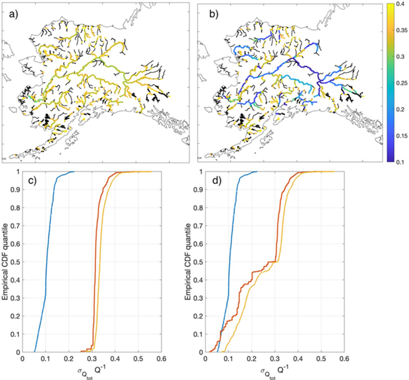
- Gage-constrained estimates should have lower systematic uncertainty; in the Alaska example, unconstrained mean flow is expected within 30%, gage-constrained mean flow within 20% near gages, and combined random plus systematic single-pass uncertainty can be as low as or lower than 35% for most reaches.
- In the Alaska example, total random error has a 67th percentile of 0.12 and more than 95% of reaches have random error less than 0.15; systematic uncertainty dominates total uncertainty for 90% of reaches in the gage-constrained domain.
Methods
- The framework uses a two-step process: Science Team algorithms estimate flow-law parameters (FLPs) via Confluence, then agencies compute discharge operationally using a modified Manning flow law with SWOT observations and ancillary data.
- Planned FLPE algorithms include reach-scale calibration (MOMMA), reach-scale inverse/McFLI methods (geoBAM/BAM, MetroMan), variational data assimilation (HiVDI, SIC4DVar), SAD, and the basin-scale MOI integrator; priors come from WBM for unconstrained and GRADES for gage-constrained products, with in situ gages used for constraints and validation.
- Example results use an end-to-end simulation with the Ohio River Community HEC-RAS model and synthetic SWOT sampling/errors, plus MOI over Alaska assuming 40% FLP systematic uncertainty, 5% flow-law approximation error, 5% gage mean annual flow uncertainty, and 0.7 inter-reach error correlation.
Limitations
- Stated: the uncertainty analysis assumes observations and flow-law approximation contribute only random error and parameters only systematic error; mapping FLP uncertainty to systematic discharge error is not trivial; McFLI algorithms do not adequately account for errors in prior mean annual flow; gage discharge itself has non-trivial uncertainty; sparse sampling may not fully resolve hydrographs, especially for smaller and flashier rivers; discharge is not computed for ice-covered rivers, lakes, dam reaches, or reaches too narrow/obstructed/unreliable in topology.
- Evident from the text: expected accuracy and uncertainty are based on simulations, algorithm intercomparison, and example domains (Alaska, Mississippi/Ohio), not on real SWOT discharge validation; the paper states results will be updated with real SWOT data and that other basins are expected to vary.
Model-written summary. Check it against the paper before relying on it.
Integrity signals
Registry
Cites
Statistics
Figures




Verification
Claims the paper makes
0 Valid · 9 Not valid · 47 Not checked · 97 Own results and interpretations
A result the paper states — it cites no source for it, so there is none to check. The quote shows it is in the paper.
In the paper
“Temporal variations in river discharge time series will be dominated by random error and are expected to be estimated within 15% for nearly all reaches, allowing accurate inference of event flow dynamics globally, including in ungaged basins.”
§ A Framework for Estimating Global River Discharge From the Surface Water and Ocean Topography Satellite Mission > Abstract
hedged- Asserted: passes — The authors put it forward as true.
- Checkable: passes — It can be checked against evidence.
- Load-bearing: passes — The paper’s conclusions depend on it.
- Based: passes — The paper gives a reason why it holds.
A result the paper states — it cites no source for it, so there is none to check. The quote shows it is in the paper.
In the paper
“We expect that discharge uncertainty will be less than 30% for two-thirds of global reaches and will be dominated by bias.”
§ A Framework for Estimating Global River Discharge From the Surface Water and Ocean Topography Satellite Mission > Abstract
hedged- Asserted: passes — The authors put it forward as true.
- Checkable: passes — It can be checked against evidence.
- Load-bearing: passes — The paper’s conclusions depend on it.
- Based: passes — The paper gives a reason why it holds.
A result the paper states — it cites no source for it, so there is none to check. The quote shows it is in the paper.
In the paper
“We expect that discharge uncertainty will be less than 30% for two-thirds of global reaches and will be dominated by bias.”
- Also stated in: § 2. SWOT Discharge Philosophy · plain
“two-thirds of global reaches and will be dominated by a systematic bias.”
§ A Framework for Estimating Global River Discharge From the Surface Water and Ocean Topography Satellite Mission > Abstract
plain- Asserted: passes — The authors put it forward as true.
- Checkable: passes — It can be checked against evidence.
- Load-bearing: passes — The paper’s conclusions depend on it.
- Based: passes — The paper gives a reason why it holds.
- Also stated in: § 2. SWOT Discharge Philosophy · plain
The paper states this without a source or data behind it here, so there is nothing to check it against. The quote shows it is in the paper.
In the paper
“Temporal variations in river discharge time series will be dominated by random error and are expected to be estimated within 15% for nearly all reaches, allowing accurate inference of event flow dynamics globally, including in ungaged basins.”
§ A Framework for Estimating Global River Discharge From the Surface Water and Ocean Topography Satellite Mission > Abstract
plain- Asserted: passes — The authors put it forward as true.
- Checkable: passes — It can be checked against evidence.
- Load-bearing: passes — The paper’s conclusions depend on it.
- Based: unclear — It is unclear why the paper says it holds.
A result the paper states — it cites no source for it, so there is none to check. The quote shows it is in the paper.
In the paper
“We assert that 𝐴𝐴 𝐴𝐴 ′ 𝑡𝑡 is measured by SWOT, as it is computed in a straightforward way from SWOT WSE and river width observations (see Appendix A).”
§ A Framework for Estimating Global River Discharge From the Surface Water and Ocean Topography Satellite Mission > 2. SWOT Discharge Philosophy
plainstates a cause- Asserted: passes — The authors put it forward as true.
- Checkable: passes — It can be checked against evidence.
- Load-bearing: passes — The paper’s conclusions depend on it.
- Based: passes — The paper gives a reason why it holds.
78 more claims
Create a free account to see all 153 claims and to verify the 35 references still open.
- It may state two separate claims as one. 46
- Probably not a substantial claim. 34
Claims other papers make about this one
Each is checked against this paper’s own text: does it say what the citing paper says it does?
In the citing paper
“The results reflect version 3 of the SWOT discharge product Consensus, which is one stage in a framework explicitly designed for iterative algorithm refinement and improvement (Durand et al., 2023).”
From SWOT Discharge Accuracy Benchmarked in South America (2026) · cites this paper as Durand et al., 2023
In the citing paper
“In isolation, SWOT's simultaneous observations of river elevation, slope, and width, leading to global reach-specific estimates of discharge (Durand et al., 2023), can be expected to provide novel insights into hydrologic dynamics (Biancamaria et al., 2016).”
From Bidirectional Translations Between Observational and Topography‐Based Hydrographic Data Sets: MERIT‐Basins and the SWOT River Database (SWORD) (2025) · cites this paper as Durand et al., 2023
In the citing paper
“Despite the existence of other global river vector data sets, we opt to base our data product on MB given its existing links to a priori discharge estimates for the SWOT mission (e.g., GRADES; Durand et al., 2023;Lin et al., 2019) and its widespread application to hydrologic modeling and analysis (Collins et al., 2024;Feng et al., 2021Feng et al., , 2022;;Lin et al., 2019;Yang et al., 2021;Yin et”
From Bidirectional Translations Between Observational and Topography‐Based Hydrographic Data Sets: MERIT‐Basins and the SWOT River Database (SWORD) (2025) · cites this paper as Durand et al., 2023
In the citing paper
“The median of the absolute value of the bias is 56%, which is larger than predicted in pre‐launch studies (Durand et al., 2023)”
From A First Look at River Discharge Estimation From SWOT Satellite Observations (2025) · cites this paper as Durand et al., 2023
In the citing paper
“This level of performance, and a modest improvement in the prior bias, is well within expectations laid out prior to launch (Durand et al., 2023).”
From A First Look at River Discharge Estimation From SWOT Satellite Observations (2025) · cites this paper as Durand et al., 2023
5 more claims about this paper
Create a free account to see every claim other papers make about this one.
Self-check
Percentages, sums and reported differences re-computed from the paper’s own numbers.
Each contradiction between two passages listed here was confirmed by an independent check.
Rated minor: it would not touch a result — a value no result rests on, a p-value that stays on the same side of the significance level, or a conflict that is clerical, resolved elsewhere in the paper, or outside its own findings.
In the paper
§ A Framework for Estimating Global River Discharge From the Surface Water and Ocean Topography Satellite Mission > 5.5.3. Combined Discharge Uncertainty
“This is still true most of the time for the gage-constrained case (Figure 10d)”
§ A Framework for Estimating Global River Discharge From the Surface Water and Ocean Topography Satellite Mission > 6. Conclusion
“Cumulative distribution functions (CDFs) of random (blue), systematic (red), and total uncertainty (gold) for the (c) unconstrained and (d) unconstrained discharge estimates.”
Rated minor: it would not touch a result — a value no result rests on, a p-value that stays on the same side of the significance level, or a conflict that is clerical, resolved elsewhere in the paper, or outside its own findings.
In the paper
§ A Framework for Estimating Global River Discharge From the Surface Water and Ocean Topography Satellite Mission > 5.5.2. Systematic Discharge Uncertainty
“Figure 9c shows the comparison of the 𝐴𝐴 𝐴𝐴𝑏𝑏 𝑄𝑄 cdf for the Yukon River for the constrained and unconstrained cases.”
§ A Framework for Estimating Global River Discharge From the Surface Water and Ocean Topography Satellite Mission > 6. Conclusion
“The difference between unconstrained (blue) and constrained (red) values of 𝐴𝐴 𝐴𝐴𝑏𝑏 𝑄𝑄 for the (c) rivers north of the Yukon basin and (d) Yukon River basin.”
Rated minor: it would not touch a result — a value no result rests on, a p-value that stays on the same side of the significance level, or a conflict that is clerical, resolved elsewhere in the paper, or outside its own findings.
In the paper
§ A Framework for Estimating Global River Discharge From the Surface Water and Ocean Topography Satellite Mission > 3.2.1. Spatial Characteristics
“SWOT discharge will be produced and is expected to be of good quality for all rivers greater than 100 m.”
§ A Framework for Estimating Global River Discharge From the Surface Water and Ocean Topography Satellite Mission > 3.2.2. Temporal Characteristics
“A total of 1,360 river that reaches wider than 100 m (2% of the total) are never observed due to small gaps in SWOT coverage.”
Citations
Cites
The Global Precipitation Measurement Mission
Hou, A. Y., Kakar, R. K., Neeck, S., Azarbarzin, A. A., Kummerow, C. D., Kojima, M., Oki, R., Nakamura, K., & Iguchi, T. (2014) · Bulletin of the American Meteorological Society · doi:10.1175/bams-d-13-00164.1 · Cited by 2,766
The development and evaluation of the Earth Gravitational Model 2008 (EGM2008)
Pavlis, N. K., Holmes, S. A., Kenyon, S. C., & Factor, J. K. (2012) · Journal of Geophysical Research: Solid Earth · doi:10.1029/2011jb008916 · Cited by 2,641
MERIT Hydro: A High‐Resolution Global Hydrography Map Based on Latest Topography Dataset
Yamazaki, D., Ikeshima, D., Sosa, J., Bates, P. D., Allen, G. H., & Pavelsky, T. M. (2019) · Water Resources Research · doi:10.1029/2019wr024873 · Cited by 1,392
Self-citationUncertainty Quantification: Theory, Implementation, and Applications
Smith, R. C. (2013) · Society for Industrial and Applied Mathematics eBooks · doi:10.1137/1.9781611973228 · Cited by 1,138
American Geophysical Union, Fall Meeting 2014
Fakhruddin, S. H. M. (2014) · ResearchSpace (University of Auckland) · Cited by 995
Global extent of rivers and streams
Allen, G. H., & Pavelsky, T. M. (2018) · Science · doi:10.1126/science.aat0636 · Cited by 970
Self-citationA physically based description of floodplain inundation dynamics in a global river routing model
Yamazaki, D., Kanae, S., Kim, H., & Oki, T. (2011) · Water Resources Research · doi:10.1029/2010wr009726 · Cited by 932
Integrated Multi-satellite Retrievals for the Global Precipitation Measurement (GPM) Mission (IMERG)
Huffman, G. J., Bolvin, D. T., Braithwaite, D., Hsu, K.-L., Joyce, R. J., Kidd, C., Nelkin, E. J., Sorooshian, S., Stocker, E. F., Tan, J., et al. (2020) · Advances in Global Change Research · doi:10.1007/978-3-030-24568-9_19 · Cited by 748
Benchmarking observational uncertainties for hydrology: rainfall, river discharge and water quality
McMillan, H., Krueger, T., & Freer, J. (2012) · Hydrological Processes · doi:10.1002/hyp.9384 · Cited by 522
Global Reconstruction of Naturalized River Flows at 2.94 Million Reaches
Lin, P., Pan, M., Beck, H. E., Yang, Y., Yamazaki, D., Frasson, R., David, C. H., Durand, M., Pavelsky, T. M., Allen, G. H., et al. (2019) · Water Resources Research · doi:10.1029/2019wr025287 · Cited by 511
Self-citationThe SWOT Mission and Its Capabilities for Land Hydrology
Biancamaria, S., Lettenmaier, D. P., & Pavelsky, T. M. (2016) · Surveys in Geophysics · doi:10.1007/s10712-015-9346-y · Cited by 458
Self-citationLarge‐scale river flow archives: importance, current status and future needs
Hannah, D. M., Demuth, S., van Lanen, H. A. J., Looser, U., Prudhomme, C., Rees, G., Stahl, K., & Tallaksen, L. M. (2011) · Hydrological Processes · doi:10.1002/hyp.7794 · Cited by 405
Gleason, C. J., & Smith, L. C. (2014) · Proceedings of the National Academy of Sciences · doi:10.1073/pnas.1317606111 · Cited by 387
Self-citationAltenau, E. H., Pavelsky, T. M., Durand, M. T., Yang, X., Frasson, R. P. D. M., & Bendezu, L. (2021) · Water Resources Research · doi:10.1029/2021wr030054 · Cited by 317
Self-citationDischarge measurements at gaging stations
Turnipseed, D. P., & Sauer, V. B. (2010) · Techniques and Methods · doi:10.3133/tm3a8 · Cited by 283
KaRIn on SWOT: Characteristics of Near-Nadir Ka-Band Interferometric SAR Imagery
Fjørtoft, R., Gaudin, J.-M., Pourthié, N., Lalaurie, J., Mallet, A., Nouvel, J. F., Martinot-Lagarde, J., Oriot, H. M., Borderies, P., Ruiz, C., et al. (2013) · IEEE Transactions on Geoscience and Remote Sensing · doi:10.1109/tgrs.2013.2258402 · Cited by 249
Andreadis, K. M., Clark, E. A., Lettenmaier, D. P., & Alsdorf, D. E. (2007) · Geophysical Research Letters · doi:10.1029/2007gl029721 · Cited by 249
Durand, M., Gleason, C. J., Garambois, P. A., Bjerklie, D., Smith, L. C., Roux, H., Rodriguez, E., Bates, P. D., Pavelsky, T. M., Monnier, J., et al. (2016) · Water Resources Research · doi:10.1002/2015wr018434 · Cited by 246
Self-citationFox, J. A. (1974) · doi:10.1007/978-1-349-01792-8_7 · Cited by 234
RivWidth: A Software Tool for the Calculation of River Widths From Remotely Sensed Imagery
Pavelsky, T. M., & Smith, L. C. (2008) · IEEE Geoscience and Remote Sensing Letters · doi:10.1109/lgrs.2007.908305 · Cited by 231
Self-citationRemote Sensing of River Discharge: A Review and a Framing for the Discipline
Gleason, C., & Durand, M. (2020) · Remote Sensing · doi:10.3390/rs12071107 · Cited by 226
Self-citationZhao, G., & Gao, H. (2019) · Remote Sensing of Environment · doi:10.1016/j.rse.2019.03.015 · Cited by 224
The past and future of global river ice
Yang, X., Pavelsky, T. M., & Allen, G. H. (2020) · Nature · doi:10.1038/s41586-019-1848-1 · Cited by 221
Self-citationGlobal Maps of Streamflow Characteristics Based on Observations from Several Thousand Catchments*
Beck, H. E., de Roo, A., & van Dijk, A. I. J. M. (2015) · Journal of Hydrometeorology · doi:10.1175/jhm-d-14-0155.1 · Cited by 220
A novel framework for discharge uncertainty quantification applied to 500 UK gauging stations
Coxon, G., Freer, J., Westerberg, I. K., Wagener, T., Woods, R., & Smith, P. J. (2015) · Water Resources Research · doi:10.1002/2014wr016532 · Cited by 217
Cohen, S., Kettner, A. J., & Syvitski, J. P. M. (2014) · Global and Planetary Change · doi:10.1016/j.gloplacha.2014.01.011 · Cited by 209
A Comparison of Methods for Streamflow Uncertainty Estimation
Kiang, J. E., Gazoorian, C., McMillan, H., Coxon, G., Le Coz, J., Westerberg, I. K., Belleville, A., Sevrez, D., Sikorska, A. E., Petersen‐Øverleir, A., et al. (2018) · Water Resources Research · doi:10.1029/2018wr022708 · Cited by 205
Frasson, R. P. D. M., Pavelsky, T. M., Fonstad, M. A., Durand, M. T., Allen, G. H., Schumann, G., Lion, C., Beighley, R. E., & Yang, X. (2019) · Geophysical Research Letters · doi:10.1029/2019gl082027 · Cited by 204
Self-citationAssessing the potential global extent of SWOT river discharge observations
Pavelsky, T. M., Durand, M. T., Andreadis, K. M., Beighley, R. E., Paiva, R. C. D., Allen, G. H., & Miller, Z. F. (2014) · Journal of Hydrology · doi:10.1016/j.jhydrol.2014.08.044 · Cited by 201
Self-citationTrigg, M. A., Wilson, M. D., Bates, P. D., Horritt, M. S., Alsdorf, D. E., Forsberg, B. R., & Vega, M. C. (2009) · Journal of Hydrology · doi:10.1016/j.jhydrol.2009.06.004 · Cited by 177
Self-citationRivers and Floodplains as Key Components of Global Terrestrial Water Storage Variability
Getirana, A., Kumar, S., Girotto, M., & Rodell, M. (2017) · Geophysical Research Letters · doi:10.1002/2017gl074684 · Cited by 162
Self-citationGleason, C. J., Smith, L. C., & Lee, J. (2014) · Water Resources Research · doi:10.1002/2014wr016109 · Cited by 160
Self-citationAssimilation of virtual wide swath altimetry to improve Arctic river modeling
Biancamaria, S., Durand, M., Andreadis, K. M., Bates, P. D., Boone, A., Mognard, N. M., Rodríguez, E., Alsdorf, D. E., Lettenmaier, D. P., & Clark, E. A. (2011) · Remote Sensing of Environment · doi:10.1016/j.rse.2010.09.008 · Cited by 158
Self-citationDurand, M., Neal, J., Rodríguez, E., Andreadis, K. M., Smith, L. C., & Yoon, Y. (2014) · Journal of Hydrology · doi:10.1016/j.jhydrol.2013.12.050 · Cited by 155
Self-citationInference of effective river properties from remotely sensed observations of water surface
Garambois, P.-A., & Monnier, J. (2015) · Advances in Water Resources · doi:10.1016/j.advwatres.2015.02.007 · Cited by 149
Self-citationDurand, M., Rodriguez, E., Alsdorf, D., & Trigg, M. A. (2009) · IEEE Journal of Selected Topics in Applied Earth Observations and Remote Sensing · doi:10.1109/jstars.2009.2033453 · Cited by 145
Self-citationEstimating river bathymetry from data assimilation of synthetic SWOT measurements
Yoon, Y., Durand, M., Merry, C. J., Clark, E. A., Andreadis, K. M., & Alsdorf, D. E. (2012) · Journal of Hydrology · doi:10.1016/j.jhydrol.2012.07.028 · Cited by 142
Self-citationTime to abandon the Manning equation?
Ferguson, R. (2010) · Earth Surface Processes and Landforms · doi:10.1002/esp.2091 · Cited by 123
Satellite remote sensing estimation of river discharge: Application to the Yukon River Alaska
Bjerklie, D. M., Birkett, C. M., Jones, J. W., Carabajal, C., Rover, J. A., Fulton, J. W., & Garambois, P.-A. (2018) · Journal of Hydrology · doi:10.1016/j.jhydrol.2018.04.005 · Cited by 123
Self-citationOubanas, H., Gejadze, I., Malaterre, P. ‐., Durand, M., Wei, R., Frasson, R. P. M., & Domeneghetti, A. (2018) · Water Resources Research · doi:10.1002/2017wr021735 · Cited by 114
Self-citationBjerklie, D. M., Dingman, S., & Bolster, C. H. (2005) · Water Resources Research · doi:10.1029/2004wr003776 · Cited by 110
Self-citationKnown and unknown unknowns: uncertainty estimation in satellite remote sensing
Povey, A. C., & Grainger, R. G. (2015) · Atmospheric Measurement Techniques · doi:10.5194/amt-8-4699-2015 · Cited by 107
Hagemann, M. W., Gleason, C. J., & Durand, M. T. (2017) · Water Resources Research · doi:10.1002/2017wr021626 · Cited by 103
Self-citationAnalytical derivation of at-a-station hydraulic-geometry relations
Lawrence, D. (2007) · Journal of Hydrology · doi:10.1016/j.jhydrol.2006.09.021 · Cited by 102
Wongchuig, S., de Paiva, R. C. D., Biancamaria, S., & Collischonn, W. (2020) · Journal of Hydrology · doi:10.1016/j.jhydrol.2020.125473 · Cited by 86
de Paiva, R. C. D., Durand, M., & Hossain, F. (2014) · Water Resources Research · doi:10.1002/2014wr015618 · Cited by 81
Self-citationBonnema, M., Sikder, M. S., Hossain, F., Durand, M., Gleason, C. J., & Bjerklie, D. M. (2016) · Water Resources Research · doi:10.1002/2015wr017296 · Cited by 78
Self-citationFrasson, R. P. D. M., Wei, R., Durand, M., Minear, J. T., Domeneghetti, A., Schumann, G., Williams, B. A., Rodriguez, E., Picamilh, C., Lion, C., et al. (2017) · Water Resources Research · doi:10.1002/2017wr020887 · Cited by 70
Self-citationEstimating River Discharge With Swath Altimetry: A Proof of Concept Using AirSWOT Observations
Tuozzolo, S., Lind, G., Overstreet, B., Mangano, J., Fonstad, M., Hagemann, M., Frasson, R. P. M., Larnier, K., Garambois, P. ‐., Monnier, J., et al. (2019) · Geophysical Research Letters · doi:10.1029/2018gl080771 · Cited by 69
Self-citationGleason, C. J., & Hamdan, A. N. (2017) · The Geographical Journal · doi:10.1111/geoj.12155 · Cited by 68
Self-citationConstraining Remote River Discharge Estimation Using Reach‐Scale Geomorphology
Brinkerhoff, C. B., Gleason, C. J., Feng, D., & Lin, P. (2020) · Water Resources Research · doi:10.1029/2020wr027949 · Cited by 64
Self-citationMapping Flow‐Obstructing Structures on Global Rivers
Yang, X., Pavelsky, T. M., Ross, M. R. V., Januchowski-Hartley, S. R., Dolan, W., Altenau, E. H., Belanger, M., Byron, D., Durand, M., Dusen, I. V., et al. (2022) · Water Resources Research · doi:10.1029/2021wr030386 · Cited by 64
Self-citationRiver discharge and bathymetry estimation from SWOT altimetry measurements
Larnier, K., Monnier, J., Garambois, P.-A., & Verley, J. (2021) · Inverse Problems in Science and Engineering · doi:10.1080/17415977.2020.1803858 · Cited by 60
Self-citationFrasson, R. P. D. M., Durand, M. T., Larnier, K., Gleason, C., Andreadis, K. M., Hagemann, M., Dudley, R., Bjerklie, D., Oubanas, H., Garambois, P., et al. (2021) · Water Resources Research · doi:10.1029/2020wr028519 · Cited by 52
Self-citationEmery, C. M., Paris, A., Biancamaria, S., Boone, A., Calmant, S., Garambois, P.-A., & Santos da Silva, J. (2018) · Hydrology and Earth System Sciences · doi:10.5194/hess-22-2135-2018 · Cited by 45
Self-citationConstraining the Assimilation of SWOT Observations With Hydraulic Geometry Relations
Andreadis, K. M., Brinkerhoff, C., & Gleason, C. J. (2020) · Water Resources Research · doi:10.1029/2019wr026611 · Cited by 45
Self-citationApproximating Wetted Perimeter in Power-Law Cross Section
Strelkoff, T., & Clemmens, A. J. (2000) · Journal of Irrigation and Drainage Engineering · doi:10.1061/(asce)0733-9437(2000)126:2(98 · Cited by 44
Yoon, Y., Garambois, P., de Paiva, R. C. D., Durand, M., Roux, H., & Beighley, R. E. (2015) · Water Resources Research · doi:10.1002/2015wr017319 · Cited by 40
Self-citationEnhancing SWOT discharge assimilation through spatiotemporal correlations
Yang, Y., Lin, P., Fisher, C. K., Turmon, M., Hobbs, J., Emery, C., Reager, J. T., David, C. H., Lu, H. M., Yang, K., et al. (2019) · Remote Sensing of Environment · doi:10.1016/j.rse.2019.111450 · Cited by 34
Self-citationBjerklie, D. M., Fulton, J. W., Dingman, S. L., Canova, M. G., Minear, J. T., & Moramarco, T. (2020) · Water Resources Research · doi:10.1029/2019wr025986 · Cited by 34
Self-citationCheng, Z., Lee, K., Kim, D., Muste, M., Vidmar, P. J., & Hulme, J. (2018) · Journal of Hydrology · doi:10.1016/j.jhydrol.2018.11.021 · Cited by 33
Temporal variations in river water surface elevation and slope captured by AirSWOT
Altenau, E. H., Pavelsky, T. M., Moller, D., Pitcher, L. H., Bates, P. D., Durand, M. T., & Smith, L. C. (2019) · Remote Sensing of Environment · doi:10.1016/j.rse.2019.02.002 · Cited by 33
Self-citationTuozzolo, S., Langhorst, T., de Moraes Frasson, R. P., Pavelsky, T., Durand, M., & Schobelock, J. J. (2019) · Journal of Hydrology · doi:10.1016/j.jhydrol.2019.06.038 · Cited by 33
Self-citationGualtieri, P., Felice, S. D., Pasquino, V., & Doria, G. P. (2017) · Journal of Hydrology and Hydromechanics · doi:10.1515/johh-2017-0028 · Cited by 31
Reconciling at‐a‐Station and at‐Many‐Stations Hydraulic Geometry Through River‐Wide Geomorphology
Brinkerhoff, C., Gleason, C. J., & Ostendorf, D. W. (2019) · Geophysical Research Letters · doi:10.1029/2019gl084529 · Cited by 31
Self-citationIshitsuka, Y., Gleason, C. J., Hagemann, M. W., Beighley, E., Allen, G. H., Feng, D., Lin, P., Pan, M., Andreadis, K., & Pavelsky, T. M. (2021) · Water Resources Research · doi:10.1029/2020wr027794 · Cited by 30
Self-citationA Participatory Science Approach to Expanding Instream Infrastructure Inventories
Whittemore, A., Ross, M. R. V., Dolan, W., Langhorst, T., Yang, X., Pawar, S., Jorissen, M., Lawton, E., Januchowski‐Hartley, S., & Pavelsky, T. (2020) · Earth's Future · doi:10.1029/2020ef001558 · Cited by 29
Self-citationObserving Rivers With Varying Spatial Scales
Rodríguez, E., Durand, M., & Frasson, R. P. D. M. (2020) · Water Resources Research · doi:10.1029/2019wr026476 · Cited by 28
Self-citationLi, D., Andreadis, K. M., Margulis, S. A., & Lettenmaier, D. P. (2020) · Water Resources Research · doi:10.1029/2019wr026999 · Cited by 27
Self-citationDurand, M., Chen, C., de Moraes Frasson, R. P., Pavelsky, T. M., Williams, B., Yang, X., & Fore, A. (2020) · Remote Sensing of Environment · doi:10.1016/j.rse.2020.111883 · Cited by 26
Self-citationTracking River Flows from Space
Gleason, C., Garambois, P.-A., & Durand, M. (2017) · Eos · doi:10.1029/2017eo078085 · Cited by 23
Self-citationAdams, T. E., Chen, S., & Dymond, R. L. (2018) · Journal of Hydrologic Engineering · doi:10.1061/(asce)he.1943-5584.0001663 · Cited by 23
Underlying Fundamentals of Kalman Filtering for River Network Modeling
Emery, C., David, C. H., Andreadis, K. M., Turmon, M., Reager, J. T., Hobbs, J., Pan, M., Famiglietti, J. S., Beighley, R. E., & Rodell, M. (2020) · Journal of Hydrometeorology · doi:10.1175/jhm-d-19-0084.1 · Cited by 21
Self-citationSimple vs complex rating curves: accounting for measurement uncertainty, slope ratio and sample size
Sörengård, M., & Baldassarre, G. D. (2017) · Hydrological Sciences Journal · doi:10.1080/02626667.2017.1367397 · Cited by 16
Integrating Lateral Inflows Into a SWOT Mission River Discharge Algorithm
Nickles, C., Beighley, E., Durand, M., & Prata de Moraes Frasson, R. (2020) · Water Resources Research · doi:10.1029/2019wr026589 · Cited by 14
Self-citationSikder, M. S., Bonnema, M., Emery, C., David, C. H., Lin, P., Pan, M., Biancamaria, S., & Gierach, M. M. (2020) · Water Resources Research · doi:10.1029/2020wr029035 · Cited by 12
Self-citationFrasson, R. P. D. M. (2021) · Elsevier eBooks · doi:10.1016/b978-0-12-819412-6.00005-5 · Cited by 10
Coss, S., Durand, M., Gleason, C. J., Tebaldi, N., & Simmons, T. (2022) · Zenodo (CERN European Organization for Nuclear Research) · doi:10.5281/zenodo.7378269 · Cited by 1
Self-citation(2022) · K-State Research Exchange (Kansas State University)
Coss, S., Durand, M., Gleason, C., Tebaldi, N., & Simmons, T. (2022) · Zenodo · doi:10.5281/zenodo.7392075
Self-citation
Research works printed but not linked: 5
- JPL Internal Document, 2017, SWOT project mission performance and error budget
- JPL Internal Document, 2018, SWOT project science requirements document
- JPL Internal Document, 2020, SWOT product description: Level 2 KaRIn high rate river single pass vector product
- Riggs R. M., 2022, Using SWOT observed lake storage change to constrain river inflow and outflow discharge
- Wang J., 2021, Preliminary results for “Lakeflow”, an algorithm to improve SWOT flow‐law parameters through integrating river‐lake mass conservation. H12I‐05: Surface Water Hydrology from SWOT, NISAR, and ICESat‐2 II eLightning
Cited by
Fu, L., Pavelsky, T. M., Crétaux, J., Morrow, R. A., Farrar, J. T., Vaze, P. V., Sengenes, P., Vinogradova‐Shiffer, N., Sylvestre‐Baron, A., Picot, N., et al. (2024) · Geophysical Research Letters · doi:10.1029/2023gl107652 · Cited by 491
Self-citationA 30 m Global Flood Inundation Model for Any Climate Scenario
Wing, O. E. J., Bates, P., Quinn, N., Savage, J. T. S., Uhe, P. F., Cooper, A., Collings, T. P., Addor, N., Lord, N. S., Hatchard, S., et al. (2024) · Water Resources Research · doi:10.1029/2023wr036460 · Cited by 114
Self-citationA First Look at River Discharge Estimation From SWOT Satellite Observations
Andreadis, K. M., Coss, S. P., Durand, M., Gleason, C. J., Simmons, T. T., Tebaldi, N., Bjerklie, D. M., Brinkerhoff, C., Dudley, R. W., Gejadze, I., et al. (2025) · Geophysical Research Letters · doi:10.1029/2024gl114185 · Cited by 110
Self-citationYang, Y., Feng, D., Beck, H. E., Hu, W., Abbas, A., Sengupta, A., Monache, L. D., Hartman, R. K., Lin, P., Shen, C., et al. (2025) · Water Resources Research · doi:10.1029/2024wr039764 · Cited by 72
Self-citationPatidar, G., Indu, J., & Karmakar, S. (2025) · Geophysical Research Letters · doi:10.1029/2025gl115804 · Cited by 62
Metadata
- Authors
- Durand, M., Gleason, C. J., Pavelsky, T. M., Prata de Moraes Frasson, R., Turmon, M., David, C. H., Altenau, E. H., Tebaldi, N., Larnier, K., Monnier, J., Malaterre, P. O., Oubanas, H., Allen, G. H., Astifan, B., Brinkerhoff, C., Bates, P. D., Bjerklie, D., Coss, S., Dudley, R., Fenoglio, L., Garambois, P., Getirana, A., Lin, P., Margulis, S. A., Matte, P., Minear, J. T., Muhebwa, A., Pan, M., Peters, D., Riggs, R., Sikder, M. S., Simmons, T., Stuurman, C., Taneja, J., Tarpanelli, A., Schulze, K., Tourian, M. J., & Wang, J.
- Affiliations
- Byrd Polar and Climate Research Center (US)
- University of Massachusetts Amherst (US)
- University of North Carolina at Chapel Hill (US)
- Jet Propulsion Laboratory California Institute of Technology Pasadena CA USA
- California Institute of Technology (US)
- Space Department CS Corporation Toulouse France
- INSA Toulouse—Math. Institute of Toulosue (IMT) Toulouse France
- Centre de Coopération Internationale en Recherche Agronomique pour le Développement (FR)
- Virginia Tech (US)
- National Oceanic and Atmospheric Administration (US)
- University of Bristol (GB)
- United States Geological Survey (US)
- Department of Geodesy and Geoinformation University of Bonn Bonn Germany
- Aix-Marseille Université (FR)
- Goddard Space Flight Center (US)
- Peking University (CN)
- University of California, Los Angeles (US)
- Environment and Climate Change Canada (CA)
- Cooperative Institute for Research in Environmental Sciences (US)
- Kansas State University (US)
- Scripps Institution of Oceanography (US)
- Texas A&M University (US)
- Research Institute for Geo-Hydrological Protection (IT)
- University of Bonn (DE)
- University of Stuttgart (DE)
- Corresponding author
- Coss, Stephen
- ORCID
- Durand, Michael
- Gleason, Colin J.
- Pavelsky, Tamlin M.
- Prata de Moraes Frasson, Renato
- Turmon, Michael
- David, Cédric H.
- Altenau, Elizabeth H.
- Tebaldi, Nikki
- Larnier, Kevin
- Malaterre, Pierre Olivier
- Oubanas, Hind
- Allen, George H.
- Brinkerhoff, Craig
- Bates, Paul D.
- Bjerklie, David
- Coss, Stephen
- Dudley, Robert
- Fenoglio, Luciana
- Garambois, Pierre‐André
- Getirana, Augusto
- Lin, Peirong
- Margulis, Steven A.
- Matte, Pascal
- Minear, J. Toby
- Muhebwa, Aggrey
- Pan, Ming
- Peters, Daniel
- Riggs, Ryan
- Sikder, Md Safat
- Simmons, Travis
- Taneja, Jay
- Tarpanelli, Angelica
- Schulze, Kerstin
- Tourian, Mohammad J.
- Wang, Jida
- Venue
- Water Resources Research
- Publisher
- American Geophysical Union (AGU)
- Published
- 2023-04
- Volume
- 59
- Issue
- 4
- ISSN
- 0043-1397 (ISSN-L)
- 1944-7973
- OpenAlex
- W4361000981
- Cited by
- 184
- References
- 79
- Citations by year
- 2026: 67 · 2025: 61 · 2024: 37 · 2023: 18
- FWCI
- 13.90
- Type
- journal article
- Language
- en
- Open access
- hybrid
- doi.org
- Licence
- Locations
- Water Resources Research (publishedVersion, cc-by-nc)
- Explore Bristol Research (publishedVersion, cc-by-nc)
- VTechWorks (Virginia Tech) (submittedVersion, cc-by-nc)
- HAL (submittedVersion, cc-by-nc)
- CNR ExploRA (submittedVersion)
- NOAA Institutional Repository (submittedVersion, cc-by-nc)
- Funders
- Jet Propulsion Laboratory
- Earth Sciences Division (80NSSC20K1143, 80NSSC20K1141, 80NSSC20K1339)
- Royal Society
- Centre National d’Etudes Spatiales
- Topics
- Physical Sciences › Environmental Science › Water Science and Technology › Hydrology and Watershed Management Studies
- Physical Sciences › Environmental Science › Global and Planetary Change › Flood Risk Assessment and Management
- Physical Sciences › Environmental Science › Environmental Engineering › Soil Moisture and Remote Sensing
- Keywords
- river discharge estimation, systematic bias, random error, ungauged basins, global hydrology
About these checks
Registry, retraction, Cites and statistics results are computed, not judged, with one exception: a printed reference that no index lists is read once by a model before it counts as a citation error. Claims are extracted by a model and kept only when their quote appears verbatim in the text; each cited source is then checked, with a model’s help, for whether it says what the claim relies on. Those verdicts can be wrong — read the claim’s quote and the cited source before relying on one.
A language model drew the claims from the paper on 2026-11-18, under version 3 of the claim definition (model deepseek-v4.1-flash, prompt extract-v3).
A second model labelled each claim on 2026-11-18 (model jev-1.13-20260917, definition revision gold-guideline-v0.2).
Statistics and arithmetic are recomputed, not judged.
Confidence bands are shown only for fields calibrated on our annotated test set. None is calibrated yet, so no band is shown.
What counts as a claim ›How we measure confidence ›How we check this ›
Are you an author, or do you see a problem with this page? Request a review
Data sources
Bibliographic data: Semantic Scholar, OpenAlex, Crossref.
Contains information from the Semantic Scholar Academic Graph Datasets, made available under the ODC Attribution License (ODC-BY 1.0).
Semantic Scholar’s data is described in: Kinney, R., et al. (2023). The Semantic Scholar Open Data Platform. arXiv:2301.10140.
