

The DOI matches its Crossref record; 63 of the 63 references it cites were found in a registry or an index.
Interpretable dimensionality reduction of single cell transcriptome data with deep generative models
Open accessPublished version of a preprint
Abstract
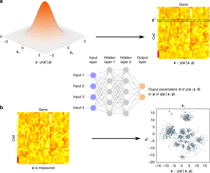
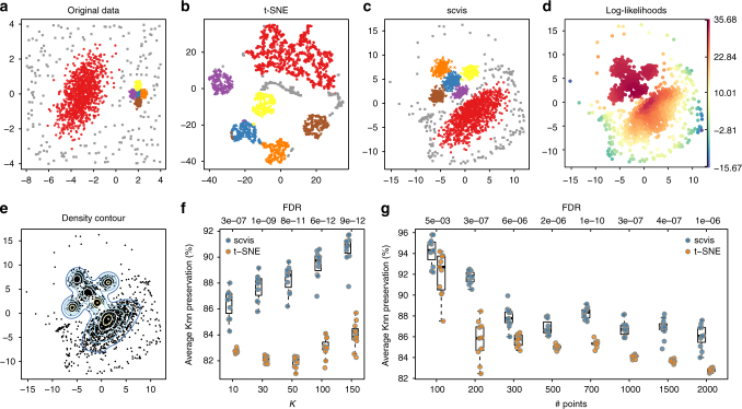
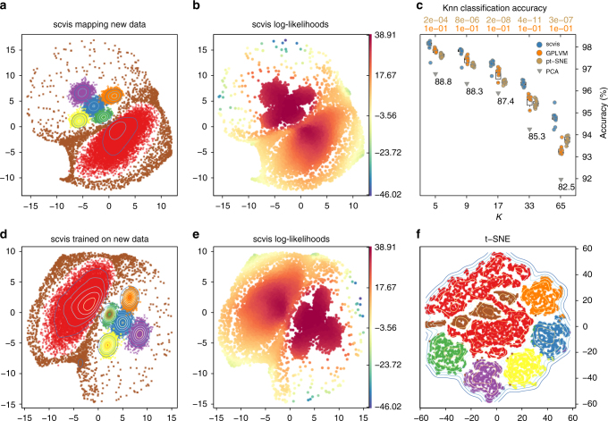
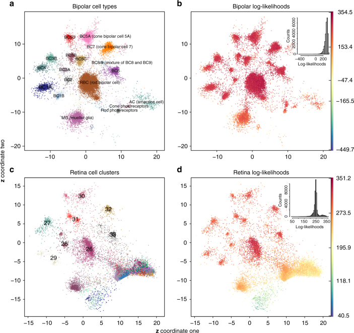
Single-cell RNA-sequencing has great potential to discover cell types, identify cell states, trace development lineages, and reconstruct the spatial organization of cells. However, dimension reduction to interpret structure in single-cell sequencing data remains a challenge. Existing algorithms are either not able to uncover the clustering structures in the data or lose global information such as groups of clusters that are close to each other. We present a robust statistical model, scvis, to capture and visualize the low-dimensional structures in single-cell gene expression data. Simulation results demonstrate that low-dimensional representations learned by scvis preserve both the local and global neighbor structures in the data. In addition, scvis is robust to the number of data points and learns a probabilistic parametric mapping function to add new data points to an existing embedding. We then use scvis to analyze four single-cell RNA-sequencing datasets, exemplifying interpretable two-dimensional representations of the high-dimensional single-cell RNA-sequencing data.
Overview
The claims and statistics of this paper haven’t been checked yet.
Run the check — free, no account needed. It reads the open-access text and checks the sources it cites.
Integrity signals
Registry
Cites
Statistics
Figures
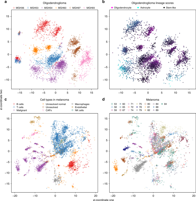
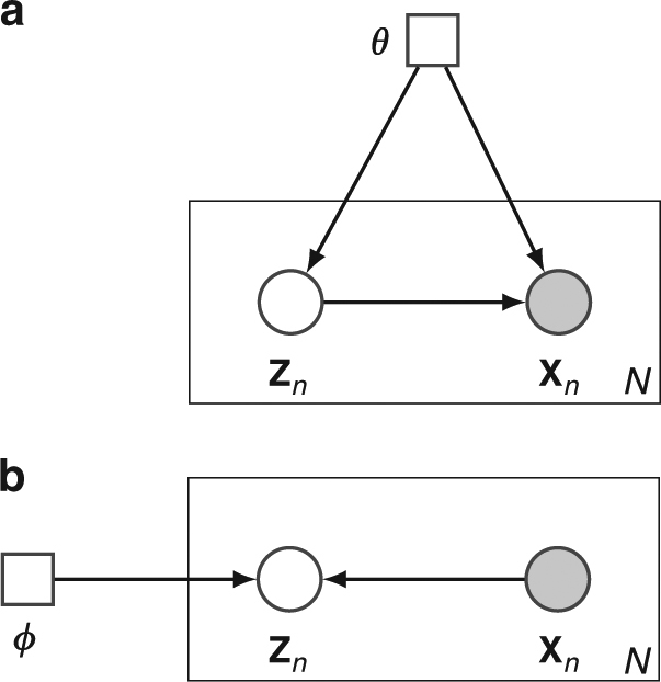
Verification
Claims the paper makes
The claims and statistics of this paper haven’t been checked yet.
Run the check — free, no account needed. It reads the open-access text and checks the sources it cites.
Claims other papers make about this one
Each is checked against this paper’s own text: does it say what the citing paper says it does?
In the citing paper
“First applications to scRNA‐seq are starting to emerge from dimensionality reduction to denoising (e.g. scVis: Ding et al, 2018; scGen: preprint: Lotfollahi et al, 2018; DCA: Eraslan et al, 2019).”
From Current best practices in single-cell RNA-seq analysis: a tutorial (2019) · cites this paper as Ding et al, 2018
Self-check
Percentages, sums and reported differences re-computed from the paper’s own numbers.
The self-check needs the paper’s full text.
Citations
Cites
Controlling the False Discovery Rate: A Practical and Powerful Approach to Multiple Testing
Benjamini, Y., & Hochberg, Y. (1995) · Journal of the Royal Statistical Society Series B: Statistical Methodology · doi:10.1111/j.2517-6161.1995.tb02031.x · Cited by 109,482
Adam: A Method for Stochastic Optimization
Kingma, D. P., & Ba, J. (2014) · arXiv · doi:10.48550/arxiv.1412.6980 · Cited by 98,946
(2008) · Journal of Machine Learning Research · Cited by 33,051
On Information and Sufficiency
Kullback, S., & Leibler, R. A. (1951) · The Annals of Mathematical Statistics · doi:10.1214/aoms/1177729694 · Cited by 20,193
(1996) · Cited by 20,179
Auto-Encoding Variational Bayes
Kingma, D. P., & Welling, M. (2013) · arXiv · doi:10.48550/arxiv.1312.6114 · Cited by 20,067
Massively parallel digital transcriptional profiling of single cells
Zheng, G. X. Y., Terry, J. M., Belgrader, P., Ryvkin, P., Bent, Z. W., Wilson, R., Ziraldo, S. B., Wheeler, T. D., McDermott, G. P., Zhu, J., et al. (2017) · Nature Communications · doi:10.1038/ncomms14049 · Cited by 7,353
Trapnell, C., Cacchiarelli, D., Grimsby, J., Pokharel, P., Li, S., Morse, M., Lennon, N. J., Livak, K. J., Mikkelsen, T. S., & Rinn, J. L. (2014) · Nature Biotechnology · doi:10.1038/nbt.2859 · Cited by 7,314
Highly parallel genome-wide expression profiling of individual cells using nanoliter droplets.
Macosko, E. Z., Basu, A., Satija, R., Nemesh, J., Shekhar, K., Goldman, M., Tirosh, I., Bialas, A. R., Kamitaki, N., Martersteck, E. M., et al. (2015) · Cell · doi:10.1016/j.cell.2015.05.002 · Cited by 7,110
limma: Linear Models for Microarray Data
Smyth, G. K. (2005) · Statistics for Biology and Health · doi:10.1007/0-387-29362-0_23 · Cited by 5,796
Research works printed but not linked: 2
- Cao, J. et al. Comprehensive single-cell transcriptional profiling of a multicellular organism. Science 357, 661–667 (2017). · DOI · Paper page
- Abadi, M. et al. TensorFlow: large-scale machine learning on heterogeneous systems. Preprint at https://static.googleusercontent.com/media/research.google.com/en//pubs/archive/45166.pdf (2015).
Cited by
Sorted by citations
Items 101–200 of 332
Deep learning-based advances and applications for single-cell RNA-sequencing data analysis
Bao, S., Li, K., Yan, C., Zhang, Z., Qu, J., & Zhou, M. (2021) · Briefings in Bioinformatics · doi:10.1093/bib/bbab473 · Cited by 40
A Survey of Autoencoder Algorithms to Pave the Diagnosis of Rare Diseases
Pratella, D., Ait-El-Mkadem, S., Bannwarth, S., Paquis‐Flucklinger, V., & Bottini, S. (2021) · International Journal of Molecular Sciences · doi:10.3390/ijms221910891 · Cited by 40
Yu, H., & Welch, J. D. (2021) · Genome Biology · doi:10.1186/s13059-021-02373-4 · Cited by 38
Deep feature extraction of single-cell transcriptomes by generative adversarial network
Bahrami, M., Maitra, M., Nagy, C., Turecki, G., Rabiee, H. R., & Li, Y. (2020) · Computer applications in the biosciences · doi:10.1093/bioinformatics/btaa976 · Cited by 38
Latent representation learning in biology and translational medicine
Kopf, A., & Claassen, M. (2021) · Patterns · doi:10.1016/j.patter.2021.100198 · Cited by 41
Artificial Intelligence in Bulk and Single-Cell RNA-Sequencing Data to Foster Precision Oncology
Giudice, M. D., Peirone, S., Perrone, S., Priante, F., Varese, F., Tirtei, E., Fagioli, F., & Cereda, M. (2021) · International Journal of Molecular Sciences · doi:10.3390/ijms22094563 · Cited by 36
Zhang, H., Zhang, J., Yuan, C., Zhang, D., Lu, D., Chen, S., Wu, Y., & Wu, C. (2024) · TrAC Trends in Analytical Chemistry · doi:10.1016/j.trac.2024.117834 · Cited by 34
Robust dimensionality reduction for data visualization with deep neural networks
Becker, M., Lippel, J., Stuhlsatz, A., & Zielke, T. (2020) · Graphical Models · doi:10.1016/j.gmod.2020.101060 · Cited by 35
Chen, S., Jiang, W., Du, Y., Yang, M., Pan, Y., Li, H., & Cui, M. (2023) · Frontiers in Genetics · doi:10.3389/fgene.2023.1276959 · Cited by 32
Deep single-cell RNA-seq data clustering with graph prototypical contrastive learning
Lee, J., Kim, S., Hyun, D., Lee, N., Kim, Y., & Park, C. (2023) · Bioinformatics · doi:10.1093/bioinformatics/btad342 · Cited by 33
Interpretable deep learning in single-cell omics
Wagle, M. M., Long, S., Chen, C., Liu, C., & Yang, P. (2024) · Bioinformatics · doi:10.1093/bioinformatics/btae374 · Cited by 32
ScCCL: Single-Cell Data Clustering Based on Self-Supervised Contrastive Learning
Du, L., Han, R., Liu, B., Wang, Y., & Li, J. (2023) · IEEE Transactions on Computational Biology and Bioinformatics · doi:10.1109/tcbb.2023.3241129 · Cited by 31
Mieth, B., Hockley, J. R. F., Görnitz, N., Vidovic, M. M.-C., Müller, K., Gutteridge, A., & Ziemek, D. (2019) · Scientific Reports · doi:10.1038/s41598-019-56911-z · Cited by 31
An efficient scRNA-seq dropout imputation method using graph attention network
Xu, C., Cai, L., & Gao, J. (2021) · BMC Bioinformatics · doi:10.1186/s12859-021-04493-x · Cited by 30
Heterostructure ZIF-8@MXene with sieving effect in mixed matrix membranes for CO2 separation
Xin, Q.-P., Kong, S.-N., Cao, X., Pan, Y., Wan, K., Chen, H., Jin, H., Gao, N.-N., Ding, X.-L., & Zhang, Y.-Z. (2024) · Separation and Purification Technology · doi:10.1016/j.seppur.2024.129779 · Cited by 30
Kinalis, S., Nielsen, F. C., Winther, O., & Bagger, F. O. (2019) · BMC Bioinformatics · doi:10.1186/s12859-019-2952-9 · Cited by 29
Brombacher, E., Hackenberg, M., Kreutz, C., Binder, H., & Treppner, M. (2022) · Frontiers in Molecular Biosciences · doi:10.3389/fmolb.2022.962644 · Cited by 30
Decision-Making with Auto-Encoding Variational BayesPreprint
Lopez, R., Boyeau, P., Yosef, N., Jordan, M. I., & Regier, J. (2020) · arXiv (Cornell University) · doi:10.48550/arxiv.2002.07217 · Cited by 30
scNODE : generative model for temporal single cell transcriptomic data prediction
Zhang, J., Larschan, E., Bigness, J., & Singh, R. (2024) · Bioinformatics · doi:10.1093/bioinformatics/btae393 · Cited by 37
Li, R., & Quon, G. (2019) · Genome biology · doi:10.1186/s13059-019-1806-0 · Cited by 30
Emerging deep learning methods for single‐cell RNA‐seq data analysis
Zheng, J., & Wang, K. (2019) · Quantitative Biology · doi:10.1007/s40484-019-0189-2 · Cited by 29
Analysis of single-cell RNA sequencing data based on autoencoders
Tangherloni, A., Ricciuti, F., Besozzi, D., Lió, P., & Cvejic, A. (2021) · BMC Bioinformatics · doi:10.1186/s12859-021-04150-3 · Cited by 30
Orrapin, S., Thongkumkoon, P., Udomruk, S., Moonmuang, S., Sutthitthasakul, S., Yongpitakwattana, P., Pruksakorn, D., & Chaiyawat, P. (2023) · International Journal of Molecular Sciences · doi:10.3390/ijms241512337 · Cited by 28
Single-cell colocalization analysis using a deep generative model
Kojima, Y., Mii, S., Hayashi, S., Hirose, H., Ishikawa, M., Akiyama, M., Enomoto, A., & Shimamura, T. (2024) · Cell Systems · doi:10.1016/j.cels.2024.01.007 · Cited by 29
Modeling regulatory networks using machine learning for systems metabolic engineering
Kwon, M. S., Lee, B. T., Lee, S. Y., & Kim, H. U. (2020) · Current Opinion in Biotechnology · doi:10.1016/j.copbio.2020.02.014 · Cited by 27
Roselin, A. G., Nanda, P., Nepal, ., & He, X. (2021) · IEEE Access · doi:10.1109/access.2021.3068172 · Cited by 27
Immunotherapy of cancer in single-cell RNA sequencing era: A precision medicine perspective
Erfanian, N., Derakhshani, A., Nasseri, S., Fereidouni, M., Baradaran, B., Tabrizi, N. J., Brunetti, O., Bernardini, R., Silvestris, N., & Safarpour, H. (2021) · Biomedicine & Pharmacotherapy · doi:10.1016/j.biopha.2021.112558 · Cited by 28
Sivaraman, V., Wu, Y., & Perer, A. (2022) · ACM International Conference on Intelligent User Interfaces (IUI) · doi:10.1145/3490099.3511137 · Cited by 27
Interpretable generative deep learning: an illustration with single cell gene expression data
Treppner, M., Binder, H., & Hess, M. (2022) · Human Genetics · doi:10.1007/s00439-021-02417-6 · Cited by 29
Synthetic single cell RNA sequencing data from small pilot studies using deep generative models
Treppner, M., Salas-Bastos, A., Hess, M., Lenz, S., Vogel, T., & Binder, H. (2021) · Scientific Reports · doi:10.1038/s41598-021-88875-4 · Cited by 26
RVAgene: generative modeling of gene expression time series data
Mitra, R., & MacLean, A. L. (2021) · Bioinformatics · doi:10.1093/bioinformatics/btab260 · Cited by 27
CALLR: a semi-supervised cell-type annotation method for single-cell RNA sequencing data
Wei, Z., & Zhang, S. (2021) · Bioinformatics · doi:10.1093/bioinformatics/btab286 · Cited by 25
Bayesian statistical learning for big data biology
Yau, C., & Campbell, K. R. (2019) · Biophysical Reviews · doi:10.1007/s12551-019-00499-1 · Cited by 25
Application of artificial intelligence in laboratory hematology: Advances, challenges, and prospects
Liao, H., Zhang, F., Chen, F., Li, Y., Sun, Y., Sloboda, D. D., Zheng, Q., Ying, B., & Hu, Y. (2025) · Acta Pharmaceutica Sinica B · doi:10.1016/j.apsb.2025.05.036 · Cited by 26
He, Y., Chen, X., Tu, N. H., & Luo, J. (2023) · IEEE Transactions on Computational Biology and Bioinformatics · doi:10.1109/tcbb.2023.3240253 · Cited by 23
Current and future perspectives of single-cell multi-omics technologies in cardiovascular research
Tan, W. L. W., Seow, W. Q., Zhang, A., Rhee, S., Wong, W. H., Greenleaf, W. J., & Wu, J. C. (2023) · Nature Cardiovascular Research · doi:10.1038/s44161-022-00205-7 · Cited by 22
Collaborative analysis for drug discovery by federated learning on non-IID data
Huang, D., Ye, X., Zhang, Y., & Sakurai, T. (2023) · Methods · doi:10.1016/j.ymeth.2023.09.001 · Cited by 22
Tyagi, N., Sharma, G., Ashraf, W., Singh, S., Singh, M. K., & Khanuja, M. (2024) · Chemical Physics Letters · doi:10.1016/j.cplett.2024.141320 · Cited by 22
Sun, Y., Kong, L., Huang, J., Deng, H., Bian, X., Li, X., Cui, F., Dou, L., Cao, C., Zou, Q., et al. (2024) · Briefings in Functional Genomics · doi:10.1093/bfgp/elae023 · Cited by 23
Tian, T., Zhong, C., Lin, X., Wei, Z., & Hakonarson, H. H. (2023) · Genome Research · doi:10.1101/gr.277068.122 · Cited by 23
Lotfollahi, M., Wolf, F. A., & Theis, F. J. (2018) · doi:10.1101/478503 · Cited by 21
Macrophage response mediated by extracellular matrix: recent progress
Xiao, W., Yang, Y., Chu, C., Rung, S., Wang, Z., Man, Y., Lin, J., & Qu, Y. (2022) · Biomedical Materials · doi:10.1088/1748-605x/aca946 · Cited by 21
An introduction to representation learning for single-cell data analysis
Gunawan, I., Vafaee, F., Meijering, E. H. W., & Lock, J. G. (2023) · Cell Reports Methods · doi:10.1016/j.crmeth.2023.100547 · Cited by 23
Analyzing Molecular Dynamics Trajectories Thermodynamically through Artificial Intelligence
Liu, X., Xing, J., Fu, H., Shao, X., & Cai, W. (2024) · Journal of Chemical Theory and Computation · doi:10.1021/acs.jctc.3c00975 · Cited by 21
K-nearest-neighbors induced topological PCA for single cell RNA-sequence data analysis
Cottrell, S., Hozumi, Y., & Wei, G. (2024) · Computers in Biology and Medicine · doi:10.1016/j.compbiomed.2024.108497 · Cited by 24
Quantifying the tradeoff between sequencing depth and cell number in single-cell RNA-seqPreprint
Svensson, V., Beltrame, E. D. V., & Pachter, L. S. (2019) · bioRxiv (Cold Spring Harbor Laboratory) · doi:10.1101/762773 · Cited by 23
Uncovering the key dimensions of high-throughput biomolecular data using deep learning
Zhang, S., Li, X., Lin, Q., Lin, J., & Wong, K. (2020) · Nucleic Acids Research · doi:10.1093/nar/gkaa191 · Cited by 20
Kužílková, D., Bugarin, C., Rejlová, K., Schulz, A. R., Mei, H. E., Paganin, M., Biffi, A., Biondi, A., Kalina, T., & Gaipa, G. (2021) · Haematologica · doi:10.3324/haematol.2021.278796 · Cited by 20
Self-Organizing Nebulous Growths for Robust and Incremental Data Visualization
Senanayake, D., Wang, W., Naik, S. H., & Halgamuge, S. K. (2020) · IEEE Transactions on Neural Networks and Learning Systems · doi:10.1109/tnnls.2020.3023941 · Cited by 19
Ding, N., Zhang, G., Zhang, L., Shen, Z., Yin, L., Zhou, S., & Deng, Y. (2023) · Computational and Structural Biotechnology Journal · doi:10.1016/j.csbj.2023.04.026 · Cited by 20
A deep learning framework for characterization of genotype data
Ausmees, K., & Nettelblad, C. (2022) · G3 Genes Genomes Genetics · doi:10.1093/g3journal/jkac020 · Cited by 21
Gundogdu, P., Loucera, C., Álamo-Álvarez, I., Dopazo, J., & Nepomuceno, I. (2022) · BioData Mining · doi:10.1186/s13040-021-00285-4 · Cited by 22
Feature importance‐based interpretation of UMAP‐visualized polymer space
Ehiro, T. (2023) · Molecular Informatics · doi:10.1002/minf.202300061 · Cited by 18
Effects of loss function and data sparsity on smooth manifold extraction with deep model
Qu, H., Zheng, J. D., & Tang, X. (2022) · Expert Systems with Applications · doi:10.1016/j.eswa.2022.116851 · Cited by 18
Machine learning to dissect perturbations in complex cellular systems
Monfort‐Lanzas, P., Rungger, K., Madersbacher, L., & Hackl, H. (2025) · Computational and Structural Biotechnology Journal · doi:10.1016/j.csbj.2025.02.028 · Cited by 20
Advances and challenges in epigenomic single-cell sequencing applications
Philpott, M., Cribbs, A. P., Brown, T. P., Brown, T. P., & Oppermann, U. C. T. (2020) · Current Opinion in Chemical Biology · doi:10.1016/j.cbpa.2020.01.013 · Cited by 19
Zhu, B., Wang, Y., Ku, L.-T., van Dijk, D., Zhang, L., Hafler, D. A., & Zhao, H. (2023) · Genome biology · doi:10.1186/s13059-023-03129-y · Cited by 18
Xu, Y., Zang, Z., Xia, J., Tan, C., Geng, Y., & Li, S. Z. (2023) · Communications Biology · doi:10.1038/s42003-023-04662-z · Cited by 17
Single-cell sequencing and its applications in bladder cancer
Wei, W., Rong, Y., Liu, S., Yang, C., Thokerunga, E., Cui, D., & Wang, F. (2022) · Expert Reviews in Molecular Medicine · doi:10.1017/erm.2021.23 · Cited by 17
Computational Methods for Single-Cell Proteomics
Guldberg, S. M., Okholm, T. L. H., McCarthy, E. E., & Spitzer, M. H. (2023) · Annual Review of Biomedical Data Science · doi:10.1146/annurev-biodatasci-020422-050255 · Cited by 18
ivis Dimensionality Reduction Framework for Biomacromolecular Simulations
Tian, H., & Tao, P. (2020) · Journal of Chemical Information and Modeling · doi:10.1021/acs.jcim.0c00485 · Cited by 16
SCDD: a novel single-cell RNA-seq imputation method with diffusion and denoising
Liu, J., Pan, Y., Ruan, Z., & Guo, J. (2022) · Briefings in Bioinformatics · doi:10.1093/bib/bbac398 · Cited by 16
Generalized EmbedSOM on quadtree-structured self-organizing maps
Kratochvíl, M., Koladiya, A., & Vondrášek, J. (2019) · F1000Research · doi:10.12688/f1000research.21642.1 · Cited by 14
Clustering Single-Cell RNA-Seq Data with Regularized Gaussian Graphical Model
Liu, Z. (2021) · Genes · doi:10.3390/genes12020311 · Cited by 14
Contrastive latent variable modeling with application to case-control sequencing experiments
Jones, A., Townes, F. W., Li, D., & Engelhardt, B. E. (2022) · The Annals of Applied Statistics · doi:10.1214/21-aoas1534 · Cited by 17
Single‐Cell and Spatial Omics: Methods and Applications
Cen, X., Huang, X., Deng, E., Gong, X., Tan, N., Ye, J. T., Wang, Y., Eils, R., Luo, Q., Li, Y., et al. (2026) · MedComm · doi:10.1002/mco2.70713 · Cited by 14
Dimensionality reduction for visualizing high-dimensional biological data
Malepathirana, T., Senanayake, D., Vidanaarachchi, R., Gautam, V., & Halgamuge, S. K. (2022) · Biosystems · doi:10.1016/j.biosystems.2022.104749 · Cited by 15
Metal-detection based techniques and their applications in metallobiology
Zhou, Y. M., Li, H., Tse, E., & Sun, H. (2024) · Chemical Science · doi:10.1039/d4sc00108g · Cited by 14
Discovering Pathway and Cell Type Signatures in Transcriptomic Compendia with Machine Learning
Way, G. P., & Greene, C. S. (2019) · Annual Review of Biomedical Data Science · doi:10.1146/annurev-biodatasci-072018-021348 · Cited by 13
Kim, G., & Chun, H. (2023) · BMC Bioinformatics · doi:10.1186/s12859-023-05552-1 · Cited by 15
Zhu, J., Li, L., TONG, J. H. M., Hui, C. W. C., Wong, C. H., Lo, K. W., Chan, R. N. C., Ai, Q. Y. H., Hui, E. P., Chan, A. T. �., et al. (2020) · PubMed Central · Cited by 13
Single-Cell RNA Sequencing Procedures and Data Analysis
Wolfien, M., David, R., & Galow, A.-M. (2021) · Exon Publications eBooks · doi:10.36255/exonpublications.bioinformatics.2021.ch2 · Cited by 16
Deep embedded clustering with multiple objectives on scRNA-seq data
Li, X., Zhang, S., & Wong, K. (2021) · Briefings in Bioinformatics · doi:10.1093/bib/bbab090 · Cited by 12
Exploring generative deep learning for omics data using log-linear models
Hess, M., Hackenberg, M., & Binder, H. (2020) · Bioinformatics · doi:10.1093/bioinformatics/btaa623 · Cited by 12
A deep generative model for gene expression profiles from single-cell RNA sequencingPreprint
Lopez, R., Regier, J., Cole, M. B., Jordan, M. I., & Yosef, N. (2017) · arXiv (Cornell University) · doi:10.48550/arxiv.1709.02082 · Cited by 12
Building interpretable predictive models with context-aware evolutionary learning
Tran, B., Sudusinghe, C., Nguyen, S., & Alahakoon, D. (2022) · Applied Soft Computing · doi:10.1016/j.asoc.2022.109854 · Cited by 11
Applications and Challenges of Machine Learning to Enable Realistic Cellular Simulations
Vasan, R., Rowan, M. P., Lee, C. T., Johnson, G. R., Rangamani, P., & Holst, M. (2020) · Frontiers in Physics · doi:10.3389/fphy.2019.00247 · Cited by 11
Semi-Supervised Deep Learning for Cell Type Identification From Single-Cell Transcriptomic Data
Dong, X., Chowdhury, S., Victor, U., Li, X., & Qian, L. (2022) · IEEE Transactions on Computational Biology and Bioinformatics · doi:10.1109/tcbb.2022.3173587 · Cited by 11
NeuroDAVIS: A neural network model for data visualization
Maitra, C., Seal, D. B., & De, R. K. (2024) · Neurocomputing · doi:10.1016/j.neucom.2023.127182 · Cited by 10
Unmixing Autoencoder for Image Reconstruction from Hyperspectral Data
Liu, X., Duan, C., Cai, W., & Shao, X. (2024) · Analytical Chemistry · doi:10.1021/acs.analchem.4c02720 · Cited by 10
Quadratic graph attention network (Q-GAT) for robust construction of gene regulatory network
Zhang, H., An, X., He, Q., Yao, Y., Zhang, Y., Fan, F., & Teng, Y. (2025) · Neurocomputing · doi:10.1016/j.neucom.2025.129635 · Cited by 10
Chen, M., Cheng, R., He, J., Chen, J., & Zhang, J. (2025) · Genome biology · doi:10.1186/s13059-025-03576-9 · Cited by 10
Zhang, X., Wang, Z., Zhang, C., Li, Y., Lu, S., Steffens, S., Mohanta, S. K., Weber, C., Habenicht, A. J. R., & Yin, C. (2022) · Methods in molecular biology · doi:10.1007/978-1-0716-1924-7_43 · Cited by 10
Improved downstream functional analysis of single-cell RNA-sequence data using DGAN
Pandey, D., & Perumal, O. (2023) · Scientific Reports · doi:10.1038/s41598-023-28952-y · Cited by 10
Nature-Inspired Compressed Sensing for Transcriptomic Profiling From Random Composite Measurements
Zhang, S., Li, X., Lin, Q., & Wong, K. (2019) · IEEE Transactions on Cybernetics · doi:10.1109/tcyb.2019.2951402 · Cited by 10
VPAC: Variational projection for accurate clustering of single-cell transcriptomic data
Chen, S., Hua, K., Cui, H., & Jiang, R. (2019) · BMC Bioinformatics · doi:10.1186/s12859-019-2742-4 · Cited by 10
Immunomics in Pediatric Rheumatic Diseases
Tay, S. H., Yaung, K. N., Leong, J. Y., Yeo, J. G., Arkachaisri, T., & Albani, S. (2019) · Frontiers in Medicine · doi:10.3389/fmed.2019.00111 · Cited by 9
Panchy, N. L., Watanabe, K., & Hong, T. (2021) · Frontiers in Genetics · doi:10.3389/fgene.2021.719099 · Cited by 9
Aragonés, D. G., Palomino‐Segura, M., Sicilia, J., Crainiciuc, G., Ballesteros, I., Sánchez‐Cabo, F., Hidalgo, A., & Calvo, G. F. (2023) · Computers in Biology and Medicine · doi:10.1016/j.compbiomed.2023.107827 · Cited by 8
Single‐Cell Sequencing to Unveil the Mystery of Embryonic Development
Li, Z., Lin, F., Zhong, C., Wang, S., Xue, X., & Shao, Y. (2021) · Advanced Biology · doi:10.1002/adbi.202101151 · Cited by 8
Pan, W., Long, F., & Pan, J. (2023) · BioData Mining · doi:10.1186/s13040-023-00333-1 · Cited by 8
Chen, H., Lu, Y., Dai, Z., Yang, Y., Li, Q., & Rao, Y. (2024) · Briefings in Bioinformatics · doi:10.1093/bib/bbae314 · Cited by 9
Clustering single-cell data based on a deep embedded subspace model
Wang, Z., Chen, L., Chen, H., & Wang, X. (2025) · Computational and Applied Mathematics · doi:10.1007/s40314-025-03268-x · Cited by 8
Visualizing High-Dimensional Single-Cell RNA-seq Data via Random Projections and Geodesic Distances
Vrahatis, A. G., Tasoulis, S. K., Dimitrakopoulos, G. Ν., & Plagianakos, V. P. (2019) · IEEE Conference on Computational Intelligence in Bioinformatics and Computational Biology (CIBCB) · doi:10.1109/cibcb.2019.8791482 · Cited by 9
Dambha‐Miller, H., Simpson, G., Akyea, R. K., Hounkpatin, H. O., Morrison, L. G., Gibson, J., Stokes, J., Islam, N., Chapman, A. P., Stuart, B. L., et al. (2022) · JMIR Research Protocols · doi:10.2196/34405 · Cited by 7
Wang, L., Nie, R., Zhang, J., & Cai, J. (2022) · BMC Bioinformatics · doi:10.1186/s12859-022-05098-8 · Cited by 7
Dimensionality reduction methods for extracting functional networks from large‐scale CRISPR screens
Hassan, A. Z., Ward, H. N., Rahman, M., Billmann, M., Lee, Y., & Myers, C. L. (2023) · Molecular Systems Biology · doi:10.15252/msb.202311657 · Cited by 7
Liu, X., Wang, H., & Gao, J. (2024) · Computational and Structural Biotechnology Journal · doi:10.1016/j.csbj.2023.12.027 · Cited by 7
Hackenberg, M., Brunn, N., Vogel, T., & Binder, H. (2025) · Communications Biology · doi:10.1038/s42003-025-07872-9 · Cited by 7
Integration of Multiple scRNA-Seq Datasets on the Autoencoder Latent Space
Riva, S. G., Cazzaniga, P., & Tangherloni, A. (2021) · IEEE International Conference on Bioinformatics and Biomedicine (BIBM) · doi:10.1109/bibm52615.2021.9669807 · Cited by 7
Metadata
- Authors
- Ding, J., Condon, A., & Shah, S. P.
- Affiliations
- Broad Institute (US)
- University of British Columbia (CA)
- BC Cancer Agency (CA)
- Corresponding author
- Ding, Jiarui
- Shah, Sohrab P.
- Venue
- Nature Communications
- Published
- 2018-05-21
- Volume
- 9
- Issue
- 1
- Pages
- 2002-2002
- ISSN
- 2041-1723 (ISSN-L)
- PMC
- PMC5962608
- OpenAlex
- W2949272108
- Cited by
- 337
- References
- 62
- Citations by year
- 2026: 12 · 2025: 32 · 2024: 38 · 2023: 50 · 2022: 48 · 2021: 52 · 2020: 49 · 2019: 47 · 2018: 8
- FWCI
- 13.87
- Type
- journal article
- Language
- en
- Open access
- gold
- doi.org
- Locations
- Nature Communications (publishedVersion, cc-by)
- bioRxiv (Cold Spring Harbor Laboratory) (acceptedVersion, cc-by-nc-nd)
- Europe PMC (PubMed Central) (publishedVersion, cc-by)
- PubMed Central (publishedVersion, cc-by)
- PubMed (publishedVersion)
- RePEc: Research Papers in Economics (submittedVersion)
- DOAJ (DOAJ: Directory of Open Access Journals) (submittedVersion, cc-by-sa)
- DOAJ (DOAJ: Directory of Open Access Journals) (submittedVersion)
- Funders
- Genome Canada
- Michael Smith Health Research BC
- Canada Research Chairs
- Terry Fox Research Institute
- BC Cancer Foundation
- Canadian Institutes of Health Research (143246_1, 115170_1)
- Canadian Cancer Society Research Institute (701584)
- Natural Sciences and Engineering Research Council of Canada
- Topics
- Life Sciences › Biochemistry, Genetics and Molecular Biology › Molecular Biology › Single-cell and spatial transcriptomics
- Life Sciences › Biochemistry, Genetics and Molecular Biology › Molecular Biology › Gene expression and cancer classification
- Physical Sciences › Computer Science › Computational Theory and Mathematics › Topological and Geometric Data Analysis
- Keywords
- single-cell RNA sequencing, dimensionality reduction, scVI, deep generative models, interpretable embeddings, cell clustering, probabilistic embedding, data augmentation, cell type discovery, cell state identification
- MeSH terms
- Algorithms, Animals, Cells, Humans, RNA, Software, Models, Statistical, Sequence Analysis, RNA, Databases, Nucleic Acid, Mice, Single-Cell Analysis, Transcriptome
About these checks
Registry, retraction, Cites and statistics results are computed, not judged, with one exception: a printed reference that no index lists is read once by a model before it counts as a citation error. Claims are extracted by a model and kept only when their quote appears verbatim in the text; each cited source is then checked, with a model’s help, for whether it says what the claim relies on. Those verdicts can be wrong — read the claim’s quote and the cited source before relying on one.
Statistics and arithmetic are recomputed, not judged.
Confidence bands are shown only for fields calibrated on our annotated test set. None is calibrated yet, so no band is shown.
What counts as a claim ›How we measure confidence ›How we check this ›
Are you an author, or do you see a problem with this page? Request a review
