

The DOI matches its Crossref record; 46 of the 46 references it cites were found in a registry or an index.
Batch effects removal for microbiome data via conditional quantile regression
Open accessAbstract
Batch effects in microbiome data arise from differential processing of specimens and can lead to spurious findings and obscure true signals. Strategies designed for genomic data to mitigate batch effects usually fail to address the zero-inflated and over-dispersed microbiome data. Most strategies tailored for microbiome data are restricted to association testing or specialized study designs, failing to allow other analytic goals or general designs. Here, we develop the Conditional Quantile Regression (ConQuR) approach to remove microbiome batch effects using a two-part quantile regression model. ConQuR is a comprehensive method that accommodates the complex distributions of microbial read counts by non-parametric modeling, and it generates batch-removed zero-inflated read counts that can be used in and benefit usual subsequent analyses. We apply ConQuR to simulated and real microbiome datasets and demonstrate its advantages in removing batch effects while preserving the signals of interest.
Overview
The claims and statistics of this paper haven’t been checked yet.
Free: it reads the open-access text and checks the first 5 claims that cite a source we can check. Create a free account to check every claim.
Integrity signals
Registry
Cites
Statistics
Figures
Verification
Claims the paper makes
The claims and statistics of this paper haven’t been checked yet.
Free: it reads the open-access text and checks the first 5 claims that cite a source we can check. Create a free account to check every claim.
Claims other papers make about this one
Each is checked against this paper’s own text: does it say what the citing paper says it does?
The check wasn’t confident either way, so it gives no verdict — never disputed.
In the citing paper
“Our meta-analysis of microbial sequencing data from nine independent αPD-1-treated melanoma cohorts82–88 revealed a higher abundance of pfl, a key enzyme in bacterial formate production, linked to ICI efficacy.”
From Exercise-induced microbiota metabolite enhances CD8 T cell antitumor immunity promoting immunotherapy efficacy (2025) · cites this paper as [88]
Experimental — accuracy not yet measuredIn the citing paper
“After analysis with Kraken2/Bracken2, we used ConQuR (v1.2.0)49 to correct for batch effects between studies. ConQuR was run on the OTU read count matrix using a penalized fitting strategy (logistic_lasso=T, quantile_type=“lasso”, interplt=T) with study metadata as the batch variable and the response as a covariate.”
From Gut microbiota-derived hexa-acylated lipopolysaccharides enhance cancer immunotherapy responses (2025) · cites this paper as [49]
Self-check
Percentages, sums and reported differences re-computed from the paper’s own numbers.
The self-check needs the paper’s full text.
Citations
Cites
DADA2: High–resolution sample inference from Illumina amplicon data
Callahan, B. J., McMurdie, P. J., Rosen, M. J., Han, A. W., Johnson, A. J. A., & Holmes, S. P. (2016) · Nature Methods · doi:10.1038/nmeth.3869 · Cited by 35,698 · cited 2×
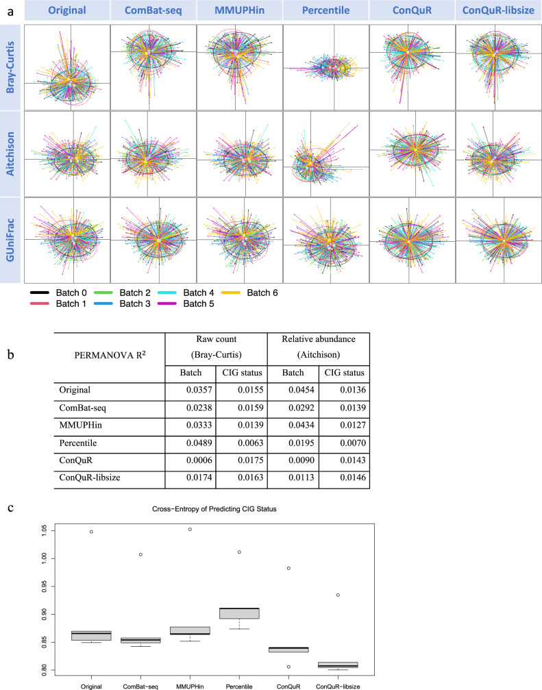
“Stool samples were collected at the Year 30 follow-up (2015 – 16) and 16S rRNA gene sequencing data were processed through DADA2 28 pipeline with Silva reference database 29 across 7 runs.”
MethodReproducible, interactive, scalable and extensible microbiome data science using QIIME 2
Bolyen, E., Rideout, J. R., Dillon, M. R., Bokulich, N. A., Abnet, C. C., Al-Ghalith, G. A., Alexander, H., Alm, E. J., Arumugam, M., Asnicar, F., et al. (2019) · Nature Biotechnology · doi:10.1038/s41587-019-0209-9 · Cited by 23,742
Koenker, R., & Bassett, G. (1978) · Econometrica · doi:10.2307/1913643 · Cited by 13,316 · cited 1×
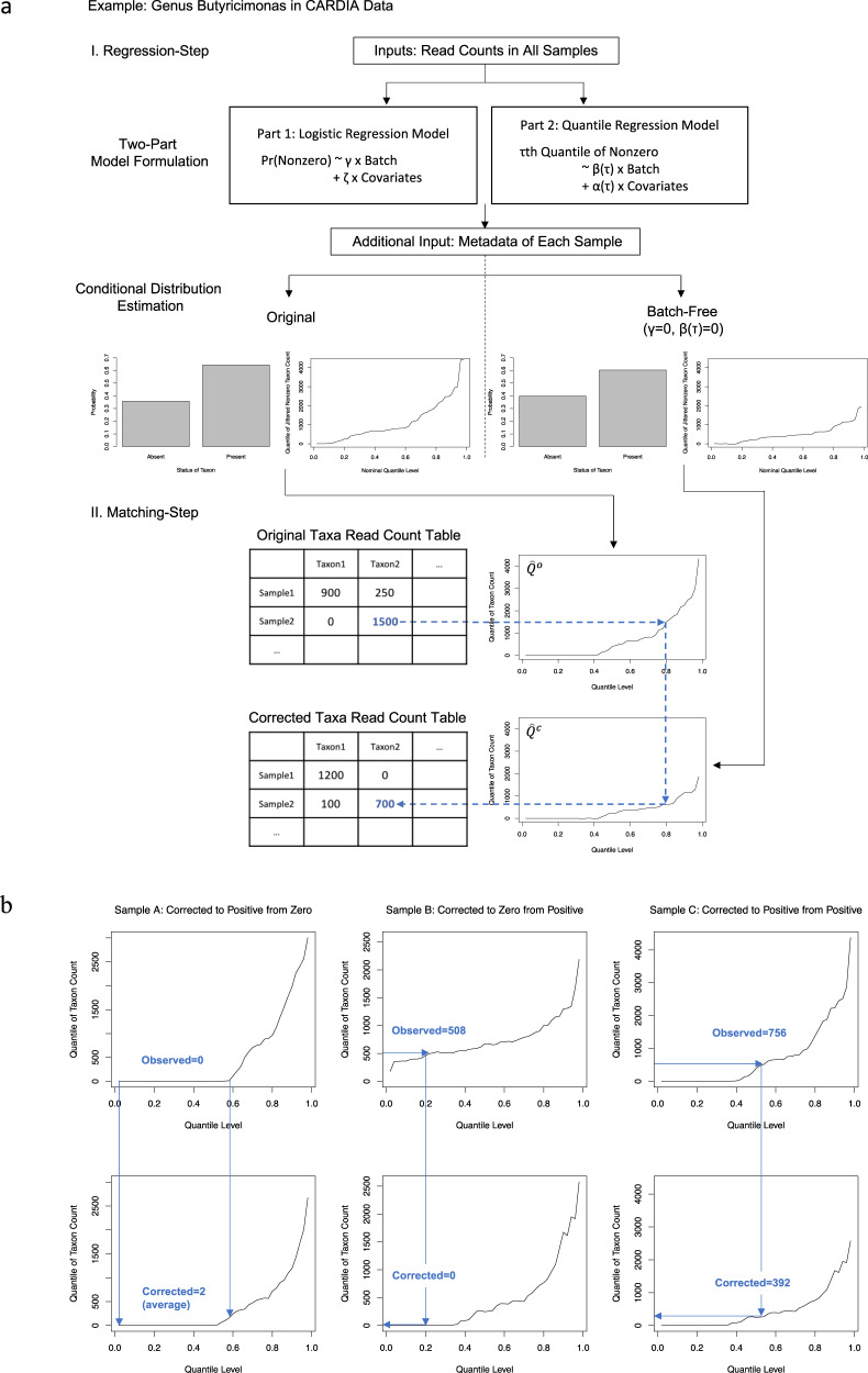
“In particular, we use quantile regression for counts 16,17 to model the read counts among samples for which the microbe is present, and separately model the presence – absence status of the microbe by logistic regression.”
MethodAdjusting batch effects in microarray expression data using empirical Bayes methods
Johnson, W. E., Li, C., & Rabinovic, A. (2007) · Biostatistics · doi:10.1093/biostatistics/kxj037 · Cited by 8,658 · cited 9×
“No DA genera associated with CIG status were found in the original, ComBat-seq, MMUPHin, Percentile, orConQuR-libsize corrected data (adjusting for HPV status, race, and sexual orientation).”
MethodInfluentialA core gut microbiome in obese and lean twins
Turnbaugh, P. J., Hamady, M., Yatsunenko, T., Cantarel, B. L., Duncan, A., Ley, R. E., Sogin, M. L., Jones, W. J., Roe, B. A., Affourtit, J. P., et al. (2009) · Nature · doi:10.1038/nature07540 · Cited by 7,823 · cited 2×
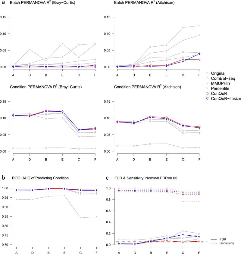
“We assessed ConQuR from three perspectives: (1) how well the batch effects are removed and condition effects are preserved, (2) the ability of corrected read counts to predict Condition, and (3) the false discovery rate (FDR) and sensitivity of subsequent individual-taxon association analysis for Condition.”
MethodA metagenome-wide association study of gut microbiota in type 2 diabetes
Qin, J., Li, Y., Cai, Z., Li, S., Zhu, J., Zhang, F., Liang, S., Zhang, W., Guan, Y., Shen, D., et al. (2012) · Nature · doi:10.1038/nature11450 · Cited by 6,762
Self-citationKoenker, R. (2005) · Cambridge University Press eBooks · doi:10.1017/cbo9780511754098 · Cited by 4,551
Circular analysis in systems neuroscience: the dangers of double dipping
Kriegeskorte, N., Simmons, W. K., Bellgowan, P. S. F., & Baker, C. I. (2009) · Nature Neuroscience · doi:10.1038/nn.2303 · Cited by 2,696 · cited 1×
“Second, ConQuR uses the meta-data twice, in both the correction and subsequent analyses, theoretically leading to over-optimism in association analysis 43 .”
MethodTackling the widespread and critical impact of batch effects in high-throughput data
Leek, J. T., Scharpf, R. B., Bravo, H. C., Simcha, D., Langmead, B., Johnson, W. E., Geman, D., Baggerly, K., & Irizarry, R. A. (2010) · Nature Reviews Genetics · doi:10.1038/nrg2825 · Cited by 2,196 · cited 1×
“Batch effects are not unique to microbiome data 9 , and standard tools have been developed for other genomic technologies, with the most commonly applied approach being ComBat 10 .”
MethodSpecification and testing of some modified count data models
Mullahy, J. (1986) · Journal of Econometrics · doi:10.1016/0304-4076(86)90002-3 · Cited by 1,870
Research works printed but not linked: 1
- Zou, H. & Yuan, M. Composite quantile regression and the oracle model selection theory. Ann. Stat. 36, 1108–1126 (2008).
Cited by
Assessing and mitigating batch effects in large-scale omics studies
Yu, Y., Mai, Y., Zheng, Y., & Shi, L. (2024) · Genome Biology · doi:10.1186/s13059-024-03401-9 · Cited by 202
“Novel methods, such as ConQuR [155] and PLSDA [156], have been specifically designed for metagenomics data.”
MethodMachine learning approaches in microbiome research: challenges and best practices
Papoutsoglou, G., Tarazona, S., Lopes, M. B., Klammsteiner, T., Ibrahimi, E., Eckenberger, J., Novielli, P., Tonda, A., Simeon, A., Shigdel, R., et al. (2023) · Frontiers in Microbiology · doi:10.3389/fmicb.2023.1261889 · Cited by 128
“To this date, only a limited number of methods exist for this purpose, and there is a general lack of established recommendations for standardized approaches (Dai et al., 2019; Ling et al., 2022; Wang and Lê Cao, 2023).”
BackgroundRegueira‐Iglesias, A., Balsa‐Castro, C., Blanco‐Pintos, T., & Tomás, I. (2023) · Molecular Oral Microbiology · doi:10.1111/omi.12434 · Cited by 154
Kumar, B., Lorusso, E., Fosso, B., & Pesole, G. (2024) · Frontiers in Microbiology · doi:10.3389/fmicb.2024.1343572 · Cited by 103
Ecological dynamics of Enterobacteriaceae in the human gut microbiome across global populations
Yin, Q., da Silva, A. C., Zorrilla, F., Almeida, A. S., Patil, K. R., & Almeida, A. (2025) · Nature Microbiology · doi:10.1038/s41564-024-01912-6 · Cited by 97
Metadata
- Authors
- Ling, W., Lu, J., Zhao, N., Lulla, A., Plantinga, A. M., Fu, W., Zhang, A., Liu, H., Song, H., Li, Z., Chen, J., Randolph, T. W., Koay, W. L. A., White, J. R., Launer, L. J., Fodor, A. A., Meyer, K. A., & Wu, M. C.
- Affiliations
- Fred Hutch Cancer Center (US)
- Johns Hopkins University (US)
- Williams College (US)
- University of Washington (US)
- University of Florida Health (US)
- Mayo Clinic (US)
- Children's National (US)
- Resphera Biosciences (US)
- National Institutes of Health (US)
- University of North Carolina at Charlotte (US)
- Corresponding author
- Zhao, Ni
- Wu, Michael C.
- ORCID
- Venue
- Nature Communications
- Published
- 2022-09-15
- Volume
- 13
- Issue
- 1
- Pages
- 5418-5418
- ISSN
- 2041-1723 (ISSN-L)
- PMC
- PMC9477887
- OpenAlex
- W4296029444
- Cited by
- 136
- References
- 46
- Citations by year
- 2026: 43 · 2025: 39 · 2024: 41 · 2023: 12 · 2022: 1
- FWCI
- 7.76
- Type
- journal article
- Language
- en
- Open access
- gold
- doi.org
- Licence
- cc-by
- creativecommons.org/licenses/by/4.0 (tdm)
- creativecommons.org/licenses/by/4.0 (vor)
- Locations
- Nature Communications (publishedVersion, cc-by)
- PubMed Central (publishedVersion, cc-by)
- PubMed (publishedVersion)
- RePEc: Research Papers in Economics (submittedVersion)
- DOAJ (DOAJ: Directory of Open Access Journals) (submittedVersion, cc-by-sa)
- Funders
- National Heart, Lung, and Blood Institute (R01HL155417, HHSN268201800004I, HHSN268201800005I, K01HL127159, and HHSN268201800007I, HHSN268201800006I, HHSN268201800007I, HHSN268201800003I)
- National Institute of General Medical Sciences (R01GM123014, R01GM129512)
- Topics
- Life Sciences › Biochemistry, Genetics and Molecular Biology › Molecular Biology › Gene expression and cancer classification
- Life Sciences › Biochemistry, Genetics and Molecular Biology › Molecular Biology › Gut microbiota and health
- Life Sciences › Biochemistry, Genetics and Molecular Biology › Molecular Biology › Genomics and Phylogenetic Studies
- Keywords
- batch effects, microbiome data, conditional quantile regression, two-part model, zero-inflated count data, overdispersion, nonparametric models, batch effect correction
- MeSH terms
- Research Design, Microbiota
About these checks
Registry, retraction, Cites and statistics results are computed, not judged, with one exception: a printed reference that no index lists is read once by a model before it counts as a citation error. Claims are extracted by a model and kept only when their quote appears verbatim in the text; each cited source is then checked, with a model’s help, for whether it says what the claim relies on. Those verdicts can be wrong — read the claim’s quote and the cited source before relying on one.
Statistics and arithmetic are recomputed, not judged.
Confidence bands are shown only for fields calibrated on our annotated test set. None is calibrated yet, so no band is shown.
What counts as a claim ›How we measure confidence ›How we check this ›
Are you an author, or do you see a problem with this page? Request a review
How to cite
Cite CoChat for the checks on this page, and the paper for its own findings.
- This page
- CoChat. (2026). Citation check: Batch effects removal for microbiome data via conditional quantile regression. https://app.cochat.ai/papers/10.1038/s41467-022-33071-9
- The paper
- Ling, W., Lu, J., Zhao, N., Lulla, A., Plantinga, A. M., Fu, W., Zhang, A., Liu, H., Song, H., Li, Z., Chen, J., Randolph, T. W., Koay, W. L. A., White, J. R., Launer, L. J., Fodor, A. A., Meyer, K. A., & Wu, M. C. (2022). Batch effects removal for microbiome data via conditional quantile regression. Nature Communications. https://doi.org/10.1038/s41467-022-33071-9
Data sources
Bibliographic data: Semantic Scholar, OpenAlex, Crossref.
Contains information from the Semantic Scholar Academic Graph Datasets, made available under the ODC Attribution License (ODC-BY 1.0).
Semantic Scholar’s data is described in: Kinney, R., et al. (2023). The Semantic Scholar Open Data Platform. arXiv:2301.10140.
