

The DOI matches its Crossref record; 3 of the 3 references it cites were found in a registry or an index.
BCM3D 2.0: accurate segmentation of single bacterial cells in dense biofilms using computationally generated intermediate image representations
Published version of a preprint
Abstract
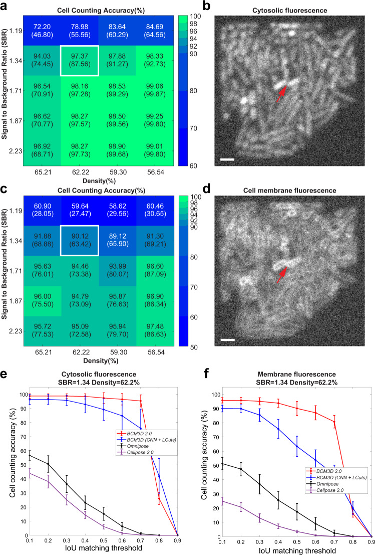
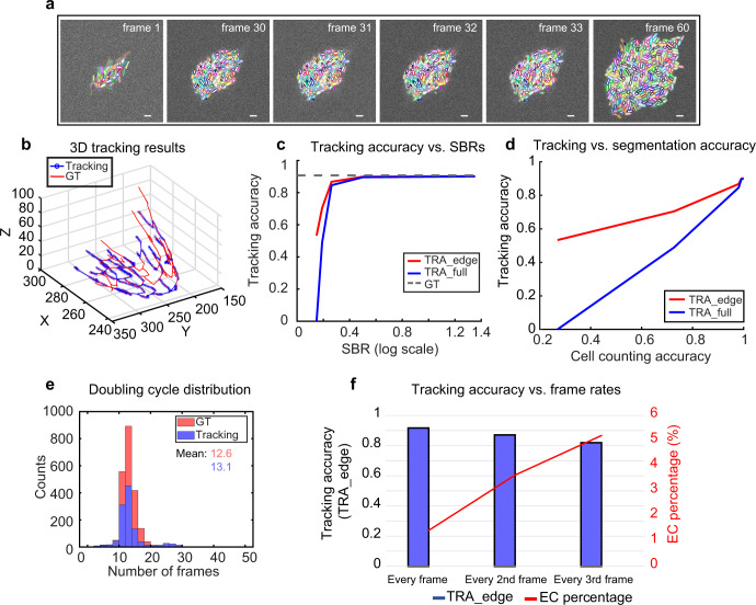
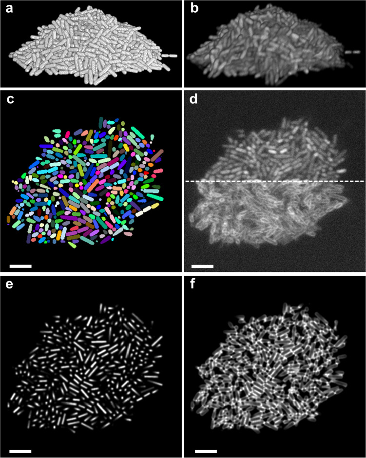
Accurate detection and segmentation of single cells in three-dimensional (3D) fluorescence time-lapse images is essential for observing individual cell behaviors in large bacterial communities called biofilms. Recent progress in machine-learning-based image analysis is providing this capability with ever-increasing accuracy. Leveraging the capabilities of deep convolutional neural networks (CNNs), we recently developed bacterial cell morphometry in 3D ( BCM3D ), an integrated image analysis pipeline that combines deep learning with conventional image analysis to detect and segment single biofilm-dwelling cells in 3D fluorescence images. While the first release of BCM3D ( BCM3D 1.0 ) achieved state-of-the-art 3D bacterial cell segmentation accuracies, low signal-to-background ratios (SBRs) and images of very dense biofilms remained challenging. Here, we present BCM3D 2.0 to address this challenge. BCM3D 2.0 is entirely complementary to the approach utilized in BCM3D 1.0 . Instead of training CNNs to perform voxel classification, we trained CNNs to translate 3D fluorescence images into intermediate 3D image representations that are, when combined appropriately, more amenable to conventional mathematical image processing than a single experimental image. Using this approach, improved segmentation results are obtained even for very low SBRs and/or high cell density biofilm images. The improved cell segmentation accuracies in turn enable improved accuracies of tracking individual cells through 3D space and time. This capability opens the door to investigating time-dependent phenomena in bacterial biofilms at the cellular level.
Overview
The claims and statistics of this paper haven’t been checked yet.
Run the check — free, no account needed. It reads the open-access text and checks the sources it cites.
Integrity signals
Registry
Cites
Statistics
Figures
Verification
Claims the paper makes
The claims and statistics of this paper haven’t been checked yet.
Run the check — free, no account needed. It reads the open-access text and checks the sources it cites.
Claims other papers make about this one
Each is checked against this paper’s own text: does it say what the citing paper says it does?
In the citing paper
“Quantitative methods, such as machine learning (ML)- and artificial intelligence (AI)-based models31-33 for image analysis and processing, may help minimize bias and improve reproducibility in biofilm quantification of wound SEM images.”
From SEMTWIST Quantification of Biofilm Infection in Human Chronic Wound Using Scanning Electron Microscopy and Machine Learning (2025) · cites this paper as [31]
Self-check
Percentages, sums and reported differences re-computed from the paper’s own numbers.
The self-check needs the paper’s full text.
Citations
Cites
Deep Residual Learning for Image Recognition
He, K., Zhang, X., Ren, S., & Sun, J. (2016) · 2016 IEEE Conference on Computer Vision and Pattern Recognition (CVPR) · doi:10.1109/cvpr.2016.90 · Cited by 235,474
Applying systems-level spectral imaging and analysis to reveal the organelle interactome
Valm, A. M., Cohen, S., Legant, W. R., Melunis, J., Hershberg, U., Wait, E., Cohen, A. R., Davidson, M. W., Betzig, E., & Lippincott-Schwartz, J. (2017) · Nature · doi:10.1038/nature22369 · Cited by 1,113
Cell Shape Dynamics in Escherichia coli
Reshes, G., Vanounou, S., Fishov, I., & Feingold, M. (2008) · Biophysical Journal · doi:10.1529/biophysj.107.104398 · Cited by 226
Research works printed but not linked: 55
- Nadell, C. D., Drescher, K. & Foster, K. R. Spatial structure, cooperation and competition in biofilms. Nat. Rev. Microbiol. 14, 589 (2016). · DOI
- Flemming, H. C. et al. Biofilms: an emergent form of bacterial life. Nat. Rev. Microbiol 14, 563–575 (2016). · DOI · Paper page
- Jayathilake, P. G. et al. A mechanistic individual-based model of microbial communities. PLoS One 12, e0181965 (2017). · DOI
- Persat, A. et al. The mechanical world of bacteria. Cell 161, 988–997 (2015). · DOI
- De la Fuente-Núñez, C., Reffuveille, F., Fernández, L. & Hancock, R. E. Bacterial biofilm development as a multicellular adaptation: antibiotic resistance and new therapeutic strategies. Curr. Opin. Microbiol. 16, 580–589 (2013). · DOI
- Frost, I. et al. Cooperation, competition and antibiotic resistance in bacterial colonies. ISME J. 12, 1582–1593 (2018). · DOI
- Yan, J. & Bassler, B. L. Surviving as a community: antibiotic tolerance and persistence in bacterial biofilms. Cell Host Microbe 26, 15–21 (2019). · DOI
- Stelzer, E. H. Light-sheet fluorescence microscopy for quantitative biology. Nat. Methods 12, 23–26 (2015). · DOI
- Power, R. M. & Huisken, J. A guide to light-sheet fluorescence microscopy for multiscale imaging. Nat. Methods 14, 360–373 (2017). · DOI
- Voleti, V. et al. Real-time volumetric microscopy of in vivo dynamics and large-scale samples with SCAPE 2.0. Nat. Methods 16, 1054–1062 (2019). · DOI · Paper page
- Mimori-Kiyosue, Y. Imaging mitotic processes in three dimensions with lattice light-sheet microscopy. Chromosome Res. 29, 37–50 (2021). · DOI
- Rosenberg, J., Cao, G., Borja-Prieto, F. & Huang, J. Lattice light-sheet microscopy multi-dimensional analyses (LaMDA) of T-cell receptor dynamics predict T-cell signaling states. Cell Syst. 10, 433–444.e435 (2020). · DOI
- Manley, H. R. et al. Frontline Science: dynamic cellular and subcellular features of migrating leukocytes revealed by in vivo lattice lightsheet microscopy. J. Leukoc. Biol. 108, 455–468 (2020). · DOI
- Yordanov, S. et al. Single-objective high-resolution confocal light sheet fluorescence microscopy for standard biological sample geometries. Biomed. Opt. Express 12, 3372–3391 (2021). · DOI
- Qin, B., et al. Cell position fates and collective fountain flow in bacterial biofilms revealed by light-sheet microscopy. Science 369, eabb8501 (2020). · DOI
- Parthasarathy, R. Monitoring microbial communities using light sheet fluorescence microscopy. Curr. Opin. Microbiol. 43, 31–37 (2018). · DOI
- Heintzmann, R. & Huser, T. Super-resolution structured illumination microscopy. Chem. Rev. 117, 13890–13908 (2017). · DOI
- Gustafsson, M. G. et al. Three-dimensional resolution doubling in wide-field fluorescence microscopy by structured illumination. Biophys. J. 94, 4957–4970 (2008). · DOI
- Weigert, M. et al. Content-aware image restoration: pushing the limits of fluorescence microscopy. Nat. Methods 15, 1090–1097 (2018). · DOI
- Chen, J. et al. Three-dimensional residual channel attention networks denoise and sharpen fluorescence microscopy image volumes. Nat. Methods 18, 678–687 (2021). · DOI
- Moen, E. et al. Deep learning for cellular image analysis. Nat Methods 16, 1233–1246 (2019). · DOI · Paper page
- Jeckel, H. & Drescher, K. Advances and opportunities in image analysis of bacterial cells and communities. FEMS Microbiol. Rev. 45, fuaa062 (2020). · DOI
- Zhang, M. et al. Non-invasive single-cell morphometry in living bacterial biofilms. Nat. Commun. 11, 6151 (2020). · DOI
- Wang, J. et al. LCuts: linear clustering of bacteria using recursive graph cuts. in 2019 IEEE International Conference on Image Processing (ICIP) 1575–1579 (IEEE, 2019). · DOI
- Stringer, C., Wang, T., Michaelos, M. & Pachitariu, M. Cellpose: a generalist algorithm for cellular segmentation. Nat. Methods 18, 100–106 (2021). · DOI · Paper page
- Weigert, M. et al. Star-convex polyhedra for 3d object detection and segmentation in microscopy. in Proceedings of the IEEE/CVF Winter Conference on Applications of Computer Vision https://arxiv.org/abs/1908.03636 (2020). · DOI
- Scherr, T., Löffler, K., Böhland, M. & Mikut, R. Cell segmentation and tracking using CNN-based distance predictions and a graph-based matching strategy. Plos One 15, e0243219 (2020). · DOI
- Meyer, F. & Beucher, S. Morphological segmentation. J. Vis. Commun. Image Represent. 1, 21–46 (1990). · DOI
- Otsu, N. A threshold selection method from gray-level histograms. IEEE Trans. Syst. Man, Cybern. 9, 62–66 (1979). · DOI
- Weigert, M. et al. Star-convex polyhedra for 3D object detection and segmentation in microscopy. in 2020 IEEE Winter Conference on Applications of Computer Vision (WACV) 3655–3662 (2020). · DOI
- Laasmaa, M., Vendelin, M. & Peterson, P. Application of regularized Richardson–Lucy algorithm for deconvolution of confocal microscopy images. J. Microsc. 243, 124–140 (2011). · DOI
- Zhang, J. et al. Optically accessible microfluidic flow channels for noninvasive high-resolution biofilm imaging using lattice light sheet microscopy. J. Phys. Chem. B 125, 12187–12196 (2021). · DOI
- Liu, R. & Jia, J. Reducing boundary artifacts in image deconvolution. in 2008 15th IEEE International Conference on Image Processing 505–508 (IEEE, 2008). · DOI
- Starck, J.-L., Pantin, E. & Murtagh, F. Deconvolution in astronomy: a review. Publ. Astron. Soc. Pac. 114, 1051 (2002). · DOI
- Wang, J. et al. Graph-theoretic post-processing of segmentation with application to dense biofilms. IEEE Trans. Image Process. 30, 8580–8594 (2021). · DOI
- Cutler, K. J., et al. Omnipose: a high-precision morphology-independent solution for bacterial cell segmentation. Nat. Methods 19, 1438–1448 (2022). · DOI
- Matula, P. et al. Cell tracking accuracy measurement based on comparison of acyclic oriented graphs. PLoS One 10, e0144959 (2015). · DOI
- Ulman, V. et al. An objective comparison of cell-tracking algorithms. Nat. Methods 14, 1141–1152 (2017). · DOI
- Wen, C. et al. 3DeeCellTracker, a deep learning-based pipeline for segmenting and tracking cells in 3D time lapse images. Elife 10, e59187 (2021). · DOI
- Magnusson, K. E., Jalden, J., Gilbert, P. M. & Blau, H. M. Global linking of cell tracks using the Viterbi algorithm. IEEE Trans. Med. Imaging 34, 911–929 (2015). · DOI
- Moen, E. et al. Accurate cell tracking and lineage construction in live-cell imaging experiments with deep learning. Preprint at https://www.biorxiv.org/content/10.1101/803205v2 (2019). · DOI
- Thormann, K. M. et al. Initial Phases of biofilm formation in Shewanella oneidensis MR-1. J. Bacteriol. 186, 8096–8104 (2004). · DOI
- Gao, R. et al. Cortical column and whole-brain imaging with molecular contrast and nanoscale resolution. Science 363, eaau8302 (2019). · DOI
- Schindelin, J. et al. Fiji: an open-source platform for biological-image analysis. Nat. Methods 9, 676–682 (2012). · DOI · Paper page
- Pettersen, E. F. et al. UCSF ChimeraX: structure visualization for researchers, educators, and developers. Protein Sci. 30, 70–82 (2021). · DOI
- Parslow, A., Cardona, A. & Bryson-Richardson, R.J. Sample drift correction following 4D confocal time-lapse imaging. J. Vis. Exp. 51086 (2014). · DOI
- Rudge, T. J., Steiner, P. J., Phillips, A. & Haseloff, J. Computational modeling of synthetic microbial biofilms. ACS Synth. Biol. 1, 345–352 (2012). · DOI
- Venkateswaran, K. et al. Polyphasic taxonomy of the genus Shewanella and description of Shewanella oneidensis sp. nov. Int. J. Syst. Bacteriol. 49, 705–724 (1999). · DOI
- Yan, T., Richardson, C. J., Zhang, M. & Gahlmann, A. Computational correction of spatially variant optical aberrations in 3D single-molecule localization microscopy. Opt. Express 27, 12582–12599 (2019). · DOI
- Liao, P.-S., Chen, T.-S. & Chung, P.-C. A fast algorithm for multilevel thresholding. J. Inf. Sci. Eng. 17, 713–727 (2001).
- Van der Walt, S. et al. scikit-image: image processing in Python. PeerJ 2, e453 (2014). · DOI
- Zunair, H., Rahman, A., Mohammed, N. & Cohen, J. P. Uniformizing techniques to process CT scans with 3D CNNs for tuberculosis prediction. in International Workshop on PRedictive Intelligence In MEdicine 156–168 (Springer, 2020). · DOI
- Jaccard, P. The distribution of the flora in the alpine zone. 1. N. Phytol. 11, 37–50 (1912). · DOI · Paper page
- Csurka, G., Larlus, D., Perronnin, F. & Meylan, F. What is a good evaluation measure for semantic segmentation? BMVC 27, 10.5244 (2013).
- Laine, R. F., Arganda-Carreras, I., Henriques, R. & Jacquemet, G. Avoiding a replication crisis in deep-learning-based bioimage analysis. Nat. Methods 18, 1136–1144 (2021). · DOI
Cited by
Sorted by citations
Singh, S., Muniz De Oliveira, F., Wang, C., Kumar, M., Xuan, Y., DeMazumder, D., Sen, C. K., & Roy, S. (2025) · Advances in Wound Care · doi:10.1089/wound.2024.0291 · Cited by 6
Metadata
- Authors
- Zhang, J., Wang, Y., Donarski, E. D., Toma, T. T., Miles, M. T., Acton, S. T., & Gahlmann, A.
- Venue
- npj Biofilms and Microbiomes
- Published
- 2022-12-18
- Volume
- 8
- Issue
- 1
- ISSN
- 2055-5008
- PMC
- PMC9760640
- Cited by
- 22
- References
- 3
- Language
- en
- Funders
- U.S. Department of Health & Human Services | NIH | National Institute of General Medical Sciences (1R01GM139002)
About these checks
Registry, retraction, Cites and statistics results are computed, not judged, with one exception: a printed reference that no index lists is read once by a model before it counts as a citation error. Claims are extracted by a model and kept only when their quote appears verbatim in the text; each cited source is then checked, with a model’s help, for whether it says what the claim relies on. Those verdicts can be wrong — read the claim’s quote and the cited source before relying on one.
Statistics and arithmetic are recomputed, not judged.
Confidence bands are shown only for fields calibrated on our annotated test set. None is calibrated yet, so no band is shown.
What counts as a claim ›How we measure confidence ›How we check this ›
Are you an author, or do you see a problem with this page? Request a review
