CoChat

Content-aware frame interpolation (CAFI): deep learning-based temporal super-resolution for fast bioimaging

Open access

Published version of a preprint

The DOI matches its Crossref record; 62 of the 62 references it cites were found in a registry or an index.

Abstract

The development of high-resolution microscopes has made it possible to investigate cellular processes in 3D and over time. However, observing fast cellular dynamics remains challenging because of photobleaching and phototoxicity. Here we report the implementation of two content-aware frame interpolation (CAFI) deep learning networks, Zooming SlowMo and Depth-Aware Video Frame Interpolation, that are highly suited for accurately predicting images in between image pairs, therefore improving the temporal resolution of image series post-acquisition. We show that CAFI is capable of understanding the motion context of biological structures and can perform better than standard interpolation methods. We benchmark CAFI’s performance on 12 different datasets, obtained from four different microscopy modalities, and demonstrate its capabilities for single-particle tracking and nuclear segmentation. CAFI potentially allows for reduced light exposure and phototoxicity on the sample for improved long-term live-cell imaging. The models and the training and testing data are available via the ZeroCostDL4Mic platform.

Overview

The claims and statistics of this paper haven’t been checked yet.

Free: it reads the open-access text and checks the first 5 claims that cite a source we can check. Create a free account to check every claim.

A few free checks a day · papers already verified open instantly · results are public

Integrity signals

Registry

Crossref · 10.1038/s41592-023-02138-w

Cites

62 of 62 references verified0 citation errors · 0 not checkable

Statistics

Figures

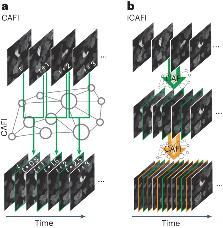
Fig. 1 Schematic representation of CAFI. a, CAFI can interpolate images between consecutive frames in a time-course dataset, therefore doubling the resulting temporal frequency. b, iCAFI allows for further improvement of the temporal resolution by repeatedly applying the network prediction.
Fig. 1 Schematic representation of CAFI. a, CAFI can interpolate images between consecutive frames in a time-course dataset, therefore doubling the resulting temporal frequency. b, iCAFI allows for further improvement of the temporal resolution by repeatedly applying the network prediction.CC BY · PubMed Central
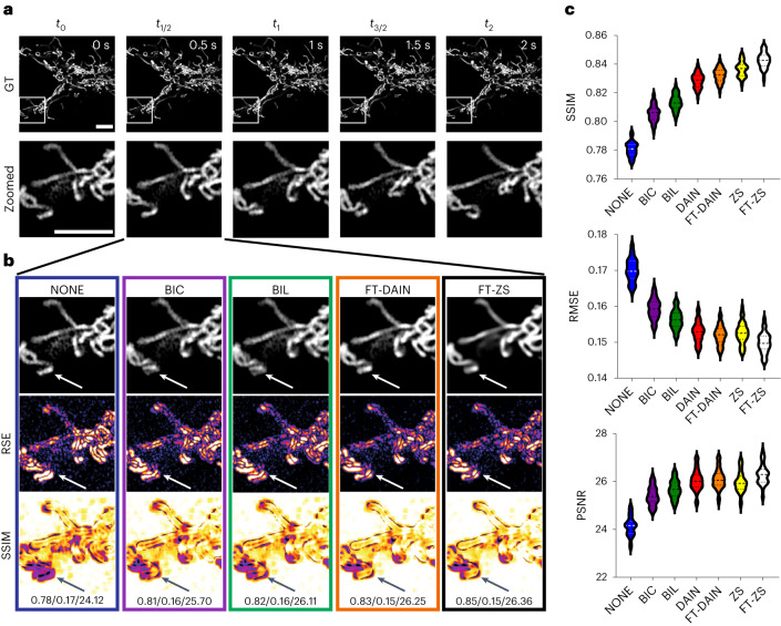
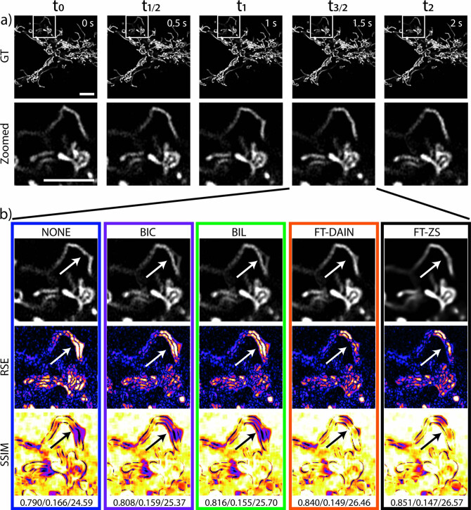
Fig. 2 CAFI enables the recovery of fast mitochondrial dynamics. a, Ground truth (GT) image sequence example (top) with zoomed-in sections (bottom) of labeled mitochondria branches of U2OS cells (scale bars, 5 μm; timestamp in top right corner of GT images). b, Interpolated frames (top), RSE maps (middle) and SSIM maps (bottom) with white/black arrows highlighting areas of fast movement; SSIM/RMSE/PSNR displayed below. c, SSIM, RMSE and PSNR metric results compared for each interpolation method including best-performing fine-tuned DAIN (FT-DAIN) and ZS (FT-ZS) networks (n = 48 interpolated image frames). Data from Fang et al.30. Source data
Fig. 2 CAFI enables the recovery of fast mitochondrial dynamics. a, Ground truth (GT) image sequence example (top) with zoomed-in sections (bottom) of labeled mitochondria branches of U2OS cells (scale bars, 5 μm; timestamp in top right corner of GT images). b, Interpolated frames (top), RSE maps (middle) and SSIM maps (bottom) with white/black arrows highlighting areas of fast movement; SSIM/RMSE/PSNR displayed below. c, SSIM, RMSE and PSNR metric results compared for each interpolation method including best-performing fine-tuned DAIN (FT-DAIN) and ZS (FT-ZS) networks (n = 48 interpolated image frames). Data from Fang et al.30. Source dataCC BY · PubMed Central
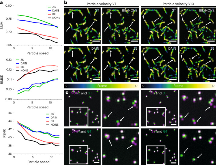
Fig. 3 Quantitative assessment of CAFI performance in predicting particle motion using simulated data. a, Image quality metrics comparison (SSIM, RMSE and PSNR) of simulated dataset interpolation with NONE, BIL, DAIN and ZS for increasing particle velocities with particle diameters of 15 pixels. These values represent the averaged metrics over the entire dataset, which comprises 17 interpolated image slices. b, Temporal color-coded overlaid projection of image sequences of the different interpolation methods for the particle velocities V7 (left) and V10 (right); white arrows highlight regions of interest for comparing interpolation performance (scale bar, 100 pixels; n = 17 frames). NONE is not displayed because of visual equivalence to BIL. c, Representative artifacts observed from predictions of NONE (SSIM 0.344, RMSE 0.203, PSNR 21.69), BIL (SSIM 0.375, RMSE 0.200, PSNR 22.58), DAIN (SSIM 0.435, RMSE 0.187, PSNR 23.82) and ZS (SSIM 0.455, RMSE 0.184, PSNR 23.57) (in magenta) overlaid with ground truth (in green) of the simulated dataset at particle velocity V7. White arrows highlight regions of interest where different techniques make mistakes (scale bars, 50 pixels). Source data
Fig. 3 Quantitative assessment of CAFI performance in predicting particle motion using simulated data. a, Image quality metrics comparison (SSIM, RMSE and PSNR) of simulated dataset interpolation with NONE, BIL, DAIN and ZS for increasing particle velocities with particle diameters of 15 pixels. These values represent the averaged metrics over the entire dataset, which comprises 17 interpolated image slices. b, Temporal color-coded overlaid projection of image sequences of the different interpolation methods for the particle velocities V7 (left) and V10 (right); white arrows highlight regions of interest for comparing interpolation performance (scale bar, 100 pixels; n = 17 frames). NONE is not displayed because of visual equivalence to BIL. c, Representative artifacts observed from predictions of NONE (SSIM 0.344, RMSE 0.203, PSNR 21.69), BIL (SSIM 0.375, RMSE 0.200, PSNR 22.58), DAIN (SSIM 0.435, RMSE 0.187, PSNR 23.82) and ZS (SSIM 0.455, RMSE 0.184, PSNR 23.57) (in magenta) overlaid with ground truth (in green) of the simulated dataset at particle velocity V7. White arrows highlight regions of interest where different techniques make mistakes (scale bars, 50 pixels). Source dataCC BY · PubMed Central
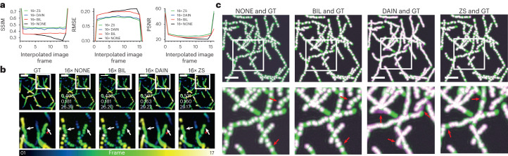
Fig. 4 iCAFI allows for 16-fold accurate interpolation of particle motion prediction. a, Image quality metrics comparison (SSIM, RMSE and PSNR) of NONE, BIL, DAIN and ZS on multistep image interpolation for every image frame between two ground truth input images. These values represent the averaged metrics over the entire dataset, which comprises 17 interpolated image slices. b, Temporal color-coded overlaid projection for visual comparison of 16× interpolated image sequences of ground truth (GT), NONE, BIL, DAIN and ZS; SSIM/RMSE/PSNR of image sequence shown in overlaid images of each interpolation technique. Red stars highlighting example of Brownian motion loss of CAFI compared with GT, and white arrows emphasizing areas of interest for interpolation discrepancies. c, Overlaid image-stack projections showing the errors between GT (green) and the interpolated results of NONE, BIL, DAIN and ZS (magenta) with matching overlaid parts (white); white boxes indicate zoomed-in sections and red arrows highlight regions of interest for error comparison (scale bars, 50 pixels; n = 17 frame). Source data
Fig. 4 iCAFI allows for 16-fold accurate interpolation of particle motion prediction. a, Image quality metrics comparison (SSIM, RMSE and PSNR) of NONE, BIL, DAIN and ZS on multistep image interpolation for every image frame between two ground truth input images. These values represent the averaged metrics over the entire dataset, which comprises 17 interpolated image slices. b, Temporal color-coded overlaid projection for visual comparison of 16× interpolated image sequences of ground truth (GT), NONE, BIL, DAIN and ZS; SSIM/RMSE/PSNR of image sequence shown in overlaid images of each interpolation technique. Red stars highlighting example of Brownian motion loss of CAFI compared with GT, and white arrows emphasizing areas of interest for interpolation discrepancies. c, Overlaid image-stack projections showing the errors between GT (green) and the interpolated results of NONE, BIL, DAIN and ZS (magenta) with matching overlaid parts (white); white boxes indicate zoomed-in sections and red arrows highlight regions of interest for error comparison (scale bars, 50 pixels; n = 17 frame). Source dataCC BY · PubMed Central
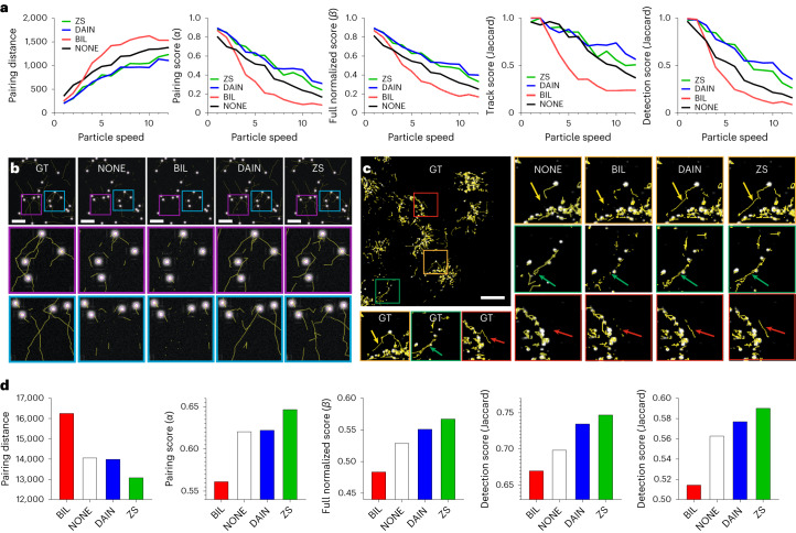
Fig. 5 Qualitative assessment of tracking performance of CAFI networks on simulated and experimental data. a, Five tracking evaluation metric results of simulated datasets at different particle velocities with NONE, BIL, DAIN and ZS interpolation. b, TrackMate tracks comparison of BIL, DAIN and ZS interpolation compared with ground truth tracks at particle velocity V10 (scale bars, 50 pixels; n = 17 frames). c, Comparison of lysosomal tracking performance on experimental lysosomal dynamics dataset with zoomed-in sections; arrows highlighting region of interest of tracking differences (scale bar, 20 μm, n = 20 frames). d, Lysosomal tracking performance metrics comparison. Source data
Fig. 5 Qualitative assessment of tracking performance of CAFI networks on simulated and experimental data. a, Five tracking evaluation metric results of simulated datasets at different particle velocities with NONE, BIL, DAIN and ZS interpolation. b, TrackMate tracks comparison of BIL, DAIN and ZS interpolation compared with ground truth tracks at particle velocity V10 (scale bars, 50 pixels; n = 17 frames). c, Comparison of lysosomal tracking performance on experimental lysosomal dynamics dataset with zoomed-in sections; arrows highlighting region of interest of tracking differences (scale bar, 20 μm, n = 20 frames). d, Lysosomal tracking performance metrics comparison. Source dataCC BY · PubMed Central
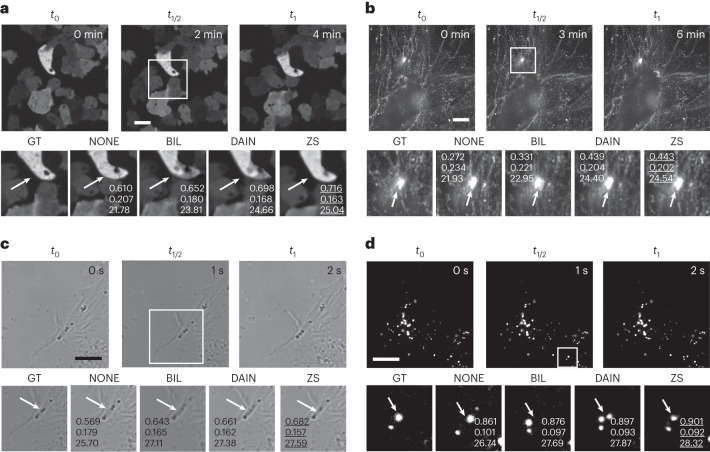
Fig. 6 CAFI allows smart interpolation for a wide range of microscopy applications. a,b, CAFI interpolation comparison of NONE, BIL, DAIN and ZS interpolation shown for D. discoideum cells (a) and fibronectin-labeled A2780 cells (b) (data from Kaukonen et al.)38, both recorded on spinning-disk confocal microscopes. c, SH-SY5Y cells recorded with a confocal brightfield microscope. d, Labeled lysosomes of SH-SY5Y cells recorded with a point-scanning confocal microscope (all scale bars, 10 μm; timestamps in top right corner of GT images); with quality metrics (SSIM/RMSE/PSNR) displayed in zoomed-in images. Arrows highlight regions of interest of visible differences between the interpolation techniques.
Fig. 6 CAFI allows smart interpolation for a wide range of microscopy applications. a,b, CAFI interpolation comparison of NONE, BIL, DAIN and ZS interpolation shown for D. discoideum cells (a) and fibronectin-labeled A2780 cells (b) (data from Kaukonen et al.)38, both recorded on spinning-disk confocal microscopes. c, SH-SY5Y cells recorded with a confocal brightfield microscope. d, Labeled lysosomes of SH-SY5Y cells recorded with a point-scanning confocal microscope (all scale bars, 10 μm; timestamps in top right corner of GT images); with quality metrics (SSIM/RMSE/PSNR) displayed in zoomed-in images. Arrows highlight regions of interest of visible differences between the interpolation techniques.CC BY · PubMed Central
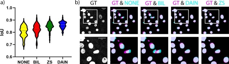
Extended Data Fig. 1 Segmentation analysis with CAFI. Segmentation analysis with CAFI: a) Comparison of the intersection of union (IoU) quality distribution of StarDist segmentation results for 4x iCAFI interpolation (DAIN, ZS) compared to classical interpolation methods (NONE, BIL) on an image sequence of labeled nuclei. The full sample comprised 66 images, and the average IoU for NONE, BIL, DAIN, and ZS was 0.80 ± 0.04, 0.82 ± 0.04, 0.86 ± 0.03, and 0.85 ± 0.03 respectively. b) One representative example for the segmentation improvements of ZS and DAIN over NONE and BIL interpolation (in cyan) compared to the ground truth segmentation (in magenta). Source data
Extended Data Fig. 1 Segmentation analysis with CAFI. Segmentation analysis with CAFI: a) Comparison of the intersection of union (IoU) quality distribution of StarDist segmentation results for 4x iCAFI interpolation (DAIN, ZS) compared to classical interpolation methods (NONE, BIL) on an image sequence of labeled nuclei. The full sample comprised 66 images, and the average IoU for NONE, BIL, DAIN, and ZS was 0.80 ± 0.04, 0.82 ± 0.04, 0.86 ± 0.03, and 0.85 ± 0.03 respectively. b) One representative example for the segmentation improvements of ZS and DAIN over NONE and BIL interpolation (in cyan) compared to the ground truth segmentation (in magenta). Source dataCC BY · PubMed Central
Extended Data Fig. 2 Table of datasets and training parameters. Training data and parameter information for fine-tuning DAIN and ZS networks for the image interpolation task of the different datasets. The other network parameters were kept as default. For datasets labeled with * the fine-tuning of DAIN did not lead to substantial improvements for this dataset and therefore the provided pretrained network was used for the comparisons. For datasets labeled with ** the fine-tuning of DAIN and ZS did not lead to substantial improvements for this dataset and therefore the provided pretrained network were used for the comparisons. The *** indicates that for the 4D datasets the frame rate displayed corresponds to the time dimension.
Extended Data Fig. 2 Table of datasets and training parameters. Training data and parameter information for fine-tuning DAIN and ZS networks for the image interpolation task of the different datasets. The other network parameters were kept as default. For datasets labeled with * the fine-tuning of DAIN did not lead to substantial improvements for this dataset and therefore the provided pretrained network was used for the comparisons. For datasets labeled with ** the fine-tuning of DAIN and ZS did not lead to substantial improvements for this dataset and therefore the provided pretrained network were used for the comparisons. The *** indicates that for the 4D datasets the frame rate displayed corresponds to the time dimension.CC BY · PubMed Central
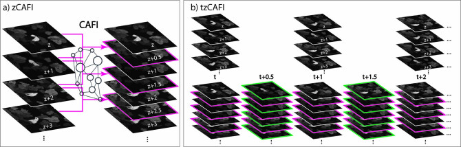
Extended Data Fig. 3 Schematic representation of two more CAFI functionalities (z-CAFI and tz-CAFI). Schematic representation of two more CAFI functionalities. a) zCAFI interpolates images between two consecutive images along the z-axis of a dataset. b) tzCAFI sequentially applies both zCAFI (a) and CAFI (Fig. 1a main text) on 4D (3D+t) dimensional dataset.
Extended Data Fig. 3 Schematic representation of two more CAFI functionalities (z-CAFI and tz-CAFI). Schematic representation of two more CAFI functionalities. a) zCAFI interpolates images between two consecutive images along the z-axis of a dataset. b) tzCAFI sequentially applies both zCAFI (a) and CAFI (Fig. 1a main text) on 4D (3D+t) dimensional dataset.CC BY · PubMed Central
Extended Data Fig. 4 2x Interpolation results on mitochondrial dynamics. 2x frame interpolation of mitochondrial dynamics image sequence of U2OS cells using classical interpolation with NONE, BIL, BIC and CAFI with fine-tuned FT-DAIN and FT-ZS. a) Ground truth (GT) image sequence example (top) with zoomed-in sections (bottom) (scale bar: 5 μm; timestamp in top right corner of GT images). b) Interpolated frame (top), RMSE map (middle) and SSIM map (bottom) with white/black arrows highlighting movement regions; SSIM/RMSE/PSNR displayed below. Data from Fang et al.30.
Extended Data Fig. 4 2x Interpolation results on mitochondrial dynamics. 2x frame interpolation of mitochondrial dynamics image sequence of U2OS cells using classical interpolation with NONE, BIL, BIC and CAFI with fine-tuned FT-DAIN and FT-ZS. a) Ground truth (GT) image sequence example (top) with zoomed-in sections (bottom) (scale bar: 5 μm; timestamp in top right corner of GT images). b) Interpolated frame (top), RMSE map (middle) and SSIM map (bottom) with white/black arrows highlighting movement regions; SSIM/RMSE/PSNR displayed below. Data from Fang et al.30.CC BY · PubMed Central
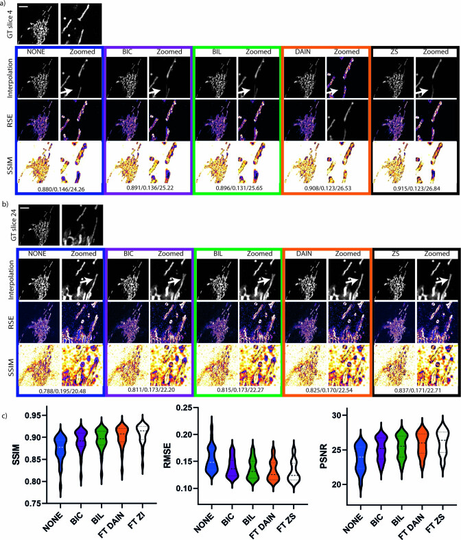
Extended Data Fig. 5 Second example of mitochondrial dynamics 2x interpolation. Interpolation analysis of second mitochondria dynamics image sequence of U2OS cells using classical interpolation with NONE, BIL, BIC and CAFI with fine-tuned FT-DAIN and FT-ZS. Interpolated frames, RMSE and SSIM images are shown of the different interpolation techniques with zoomed-in sections next to it (scale bar: 5 μm; n=29 interpolated image frames). a) Showing frame 4 and b) frame 24 of the same sequence. c) Showing violin plots of the SSIM, RMSE and PSNR error of the different simulation techniques. Data from Fang et al.30. Source data
Extended Data Fig. 5 Second example of mitochondrial dynamics 2x interpolation. Interpolation analysis of second mitochondria dynamics image sequence of U2OS cells using classical interpolation with NONE, BIL, BIC and CAFI with fine-tuned FT-DAIN and FT-ZS. Interpolated frames, RMSE and SSIM images are shown of the different interpolation techniques with zoomed-in sections next to it (scale bar: 5 μm; n=29 interpolated image frames). a) Showing frame 4 and b) frame 24 of the same sequence. c) Showing violin plots of the SSIM, RMSE and PSNR error of the different simulation techniques. Data from Fang et al.30. Source dataCC BY · PubMed Central
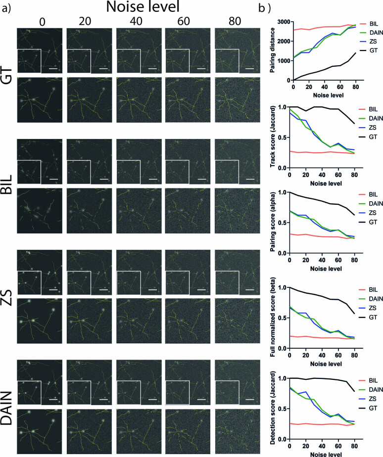
Extended Data Fig. 6 Tracking experiment on noised simulated data. Tracking of noised simulated particle dataset. a) Simulated particle dataset generated with ICY track generator40 with different levels of noise added with Fiji36 were tracked with TrackMate35 after interpolating with BIL, DAIN and ZS. GT described the comparison of the tracks of noised ground truth sequence to the real generated tracks. b) Five tracking evaluation metric results of simulated particles at different noise levels with BIL, DAIN and ZS interpolation (n=45 images averaged).
Extended Data Fig. 6 Tracking experiment on noised simulated data. Tracking of noised simulated particle dataset. a) Simulated particle dataset generated with ICY track generator40 with different levels of noise added with Fiji36 were tracked with TrackMate35 after interpolating with BIL, DAIN and ZS. GT described the comparison of the tracks of noised ground truth sequence to the real generated tracks. b) Five tracking evaluation metric results of simulated particles at different noise levels with BIL, DAIN and ZS interpolation (n=45 images averaged).CC BY · PubMed Central
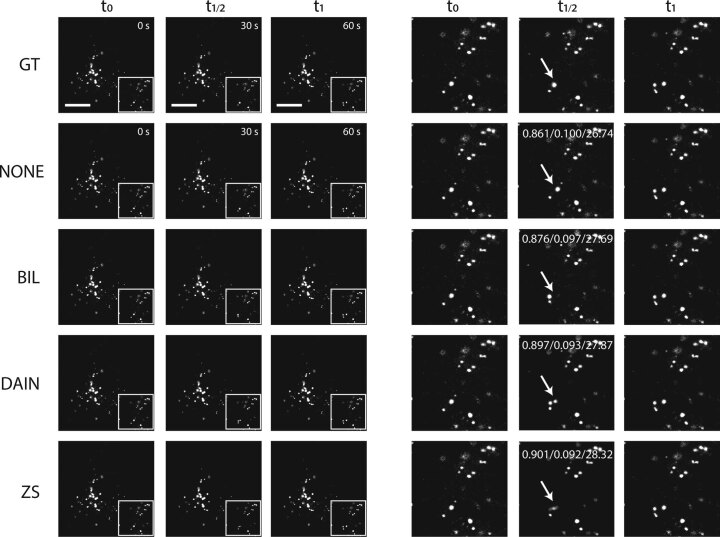
Extended Data Fig. 7 2x frame interpolation on moving lysosome of SHSY5Y cells. 2x frame interpolation of NONE, BIL, DAIN and ZS for lysosomes of SH-SY5Y cells recorded on a point-scanning confocal microscope. Overall ZS produces slightly better-quality results than DAIN even though ZS misses faster moving lysosomes which DAIN is able to capture well (example highlighted with white arrows in zoomed-in sections on the right). SSIM/RMSE/PSNR values displayed in the zoomed-in interpolated images. CAFI tools clearly outperform NONE and BIL interpolations. Scale bar: 10 μm.
Extended Data Fig. 7 2x frame interpolation on moving lysosome of SHSY5Y cells. 2x frame interpolation of NONE, BIL, DAIN and ZS for lysosomes of SH-SY5Y cells recorded on a point-scanning confocal microscope. Overall ZS produces slightly better-quality results than DAIN even though ZS misses faster moving lysosomes which DAIN is able to capture well (example highlighted with white arrows in zoomed-in sections on the right). SSIM/RMSE/PSNR values displayed in the zoomed-in interpolated images. CAFI tools clearly outperform NONE and BIL interpolations. Scale bar: 10 μm.CC BY · PubMed Central
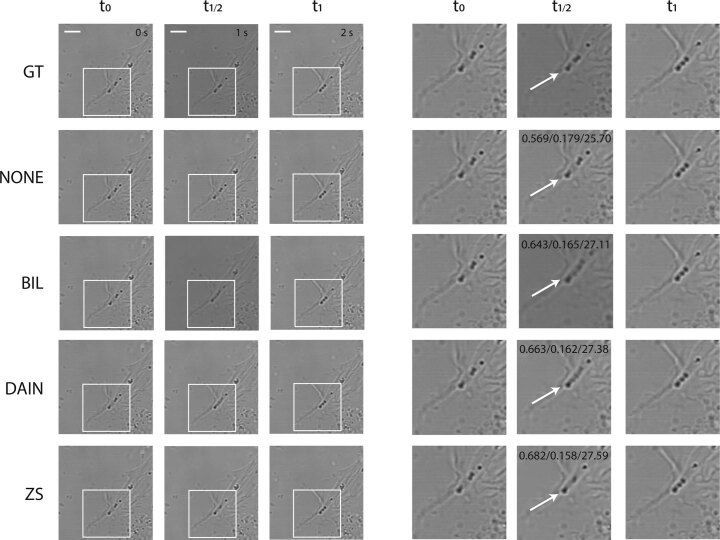
Extended Data Fig. 8 2x frame interpolation on brightfield image of SHSY5Y cells. 2x frame interpolation with NONE, BIL, DAIN and ZS for SH-SY5Y cells recorded on a confocal brightfield microscope. ZS produces slightly better-quality results than DAIN. DAIN creates visual artifacts for fast moving lipid droplets while ZS manages to capture the movement better (see white arrows in zoomed-in sections on the right). SSIM/RMSE/PSNR values displayed in the zoomed-in interpolated images. CAFI tools clearly outperform NONE and BIL interpolations. Scale bar: 10 μm.
Extended Data Fig. 8 2x frame interpolation on brightfield image of SHSY5Y cells. 2x frame interpolation with NONE, BIL, DAIN and ZS for SH-SY5Y cells recorded on a confocal brightfield microscope. ZS produces slightly better-quality results than DAIN. DAIN creates visual artifacts for fast moving lipid droplets while ZS manages to capture the movement better (see white arrows in zoomed-in sections on the right). SSIM/RMSE/PSNR values displayed in the zoomed-in interpolated images. CAFI tools clearly outperform NONE and BIL interpolations. Scale bar: 10 μm.CC BY · PubMed Central
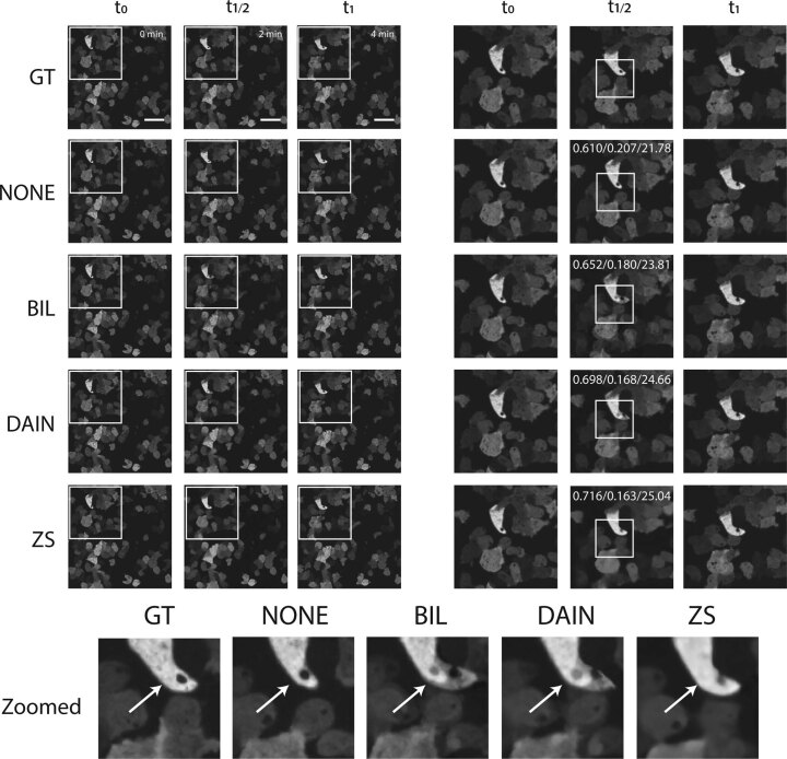
Extended Data Fig. 9 2x frame interpolation on moving Dictyostelium discoideum cells. 2x image frame interpolation of NONE, BIL, DAIN and ZS for Dictyostelium discoideum cells recorded on a spinning-disk confocal microscope. ZS creates smoother transitions and better-quality interpolation results than DAIN (see white arrow in zoomed-in section). SSIM/RMSE/PSNR values displayed in the zoomed-in interpolated images. CAFI tools clearly outperform NONE and BIL interpolations. Scale bar: 20 μm.
Extended Data Fig. 9 2x frame interpolation on moving Dictyostelium discoideum cells. 2x image frame interpolation of NONE, BIL, DAIN and ZS for Dictyostelium discoideum cells recorded on a spinning-disk confocal microscope. ZS creates smoother transitions and better-quality interpolation results than DAIN (see white arrow in zoomed-in section). SSIM/RMSE/PSNR values displayed in the zoomed-in interpolated images. CAFI tools clearly outperform NONE and BIL interpolations. Scale bar: 20 μm.CC BY · PubMed Central
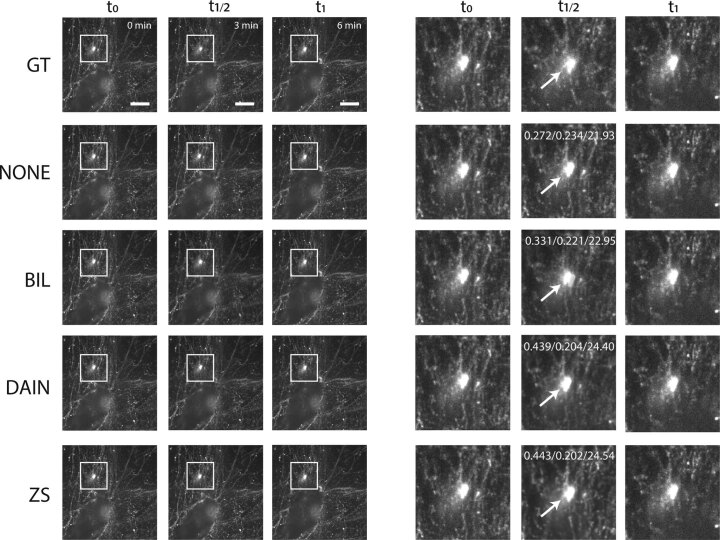
Extended Data Fig. 10 2x frame interpolation on fibronectin labelled A2780 cells. 2x image frame interpolation of NONE, BIL, DAIN and ZS for fibronectin labelled A2780 cells recorded on a spinning-disk confocal microscope. ZS creates smoother transitions and better-quality interpolation results than DAIN (see white arrow in zoomed-in sections on the right). SSIM/RMSE/PSNR values displayed in the zoomed-in interpolated images. CAFI tools clearly outperform NONE and BIL interpolations. Scale bar: 10 μm. Data from Kaukonen et al.38.
Extended Data Fig. 10 2x frame interpolation on fibronectin labelled A2780 cells. 2x image frame interpolation of NONE, BIL, DAIN and ZS for fibronectin labelled A2780 cells recorded on a spinning-disk confocal microscope. ZS creates smoother transitions and better-quality interpolation results than DAIN (see white arrow in zoomed-in sections on the right). SSIM/RMSE/PSNR values displayed in the zoomed-in interpolated images. CAFI tools clearly outperform NONE and BIL interpolations. Scale bar: 10 μm. Data from Kaukonen et al.38.CC BY · PubMed Central

Verification

Claims the paper makes

The claims and statistics of this paper haven’t been checked yet.

Free: it reads the open-access text and checks the first 5 claims that cite a source we can check. Create a free account to check every claim.

A few free checks a day · papers already verified open instantly · results are public

Claims other papers make about this one

Each is checked against this paper’s own text: does it say what the citing paper says it does?

Self-check

Percentages, sums and reported differences re-computed from the paper’s own numbers.

The self-check needs the paper’s full text.

Citations

Cites

Show all 62 references

Cited by

See all 49

Metadata

Authors
Priessner, M., Gaboriau, D. C. A., Sheridan, A., Lenn, T., Garzon-Coral, C., Dunn, A. R., Chubb, J. R., Tousley, A. M., Majzner, R. G., Manor, U., Vilar, R., & Laine, R. F.
Affiliations
  • Imperial College London (GB)
  • Salk Institute for Biological Studies (US)
  • University College London (GB)
  • Stanford Medicine (US)
  • MRC Laboratory for Molecular Cell Biology (GB)
  • Stanford University (US)
Corresponding author
  • Priessner, Martin
  • Laine, Romain F.
Venue
Nature Methods
Published
2024-01-18
Volume
21
Issue
2
Pages
322-330
ISSN
  • 1548-7091 (ISSN-L)
  • 1548-7105
OpenAlex
W4390975819
Cited by
35
References
54
Citations by year
2026: 9 · 2025: 18 · 2024: 8
FWCI
4.86
Type
journal article
Language
en
Open access
Licence
Locations
  • Nature Methods (publishedVersion, cc-by)
  • PubMed Central (publishedVersion, cc-by)
  • PubMed (publishedVersion)
  • eScholarship (California Digital Library) (submittedVersion, cc-by)
Funders
  • National Science Foundation (2014862)
  • Wellcome Trust (104931/Z/14/Z, 104931, BB/L015129/1, 202867/Z/16/Z)
  • Imperial College London (BB/L015129/1, 104931/Z/14/Z)
  • National Institutes of Health
  • Medical Research Council (MR/T027924/1)
  • Engineering and Physical Sciences Research Council (EP/L016737/1, 1816855, EP/J021199/1)
  • Biotechnology and Biological Sciences Research Council (BB/L015129/1, L015129)
  • National Institute on Aging (P30AG068635)
  • National Cancer Institute
  • National Institute of General Medical Sciences (R35GM130332)
Topics
  • Physical Sciences › Computer Science › Computer Vision and Pattern Recognition › Advanced Image Processing Techniques
  • Life Sciences › Biochemistry, Genetics and Molecular Biology › Biophysics › Cell Image Analysis Techniques
  • Life Sciences › Biochemistry, Genetics and Molecular Biology › Biophysics › Advanced Fluorescence Microscopy Techniques
Keywords
temporal super-resolution, frame interpolation, photobleaching, phototoxicity, single-particle tracking, nuclei segmentation, live-cell imaging
MeSH terms
Single Molecule Imaging, Deep Learning, Microscopy, Motion

About these checks

Registry, retraction, Cites and statistics results are computed, not judged, with one exception: a printed reference that no index lists is read once by a model before it counts as a citation error. Claims are extracted by a model and kept only when their quote appears verbatim in the text; each cited source is then checked, with a model’s help, for whether it says what the claim relies on. Those verdicts can be wrong — read the claim’s quote and the cited source before relying on one.

Statistics and arithmetic are recomputed, not judged.

Confidence bands are shown only for fields calibrated on our annotated test set. None is calibrated yet, so no band is shown.

What counts as a claim ›How we measure confidence ›How we check this ›

Are you an author, or do you see a problem with this page? Request a review

How to cite

Cite CoChat for the checks on this page, and the paper for its own findings.

This page
CoChat. (2026). Citation check: Content-aware frame interpolation (CAFI): deep learning-based temporal super-resolution for fast bioimaging. https://app.cochat.ai/papers/10.1038/s41592-023-02138-w
The paper
Priessner, M., Gaboriau, D. C. A., Sheridan, A., Lenn, T., Garzon-Coral, C., Dunn, A. R., Chubb, J. R., Tousley, A. M., Majzner, R. G., Manor, U., Vilar, R., & Laine, R. F. (2024). Content-aware frame interpolation (CAFI): deep learning-based temporal super-resolution for fast bioimaging. Nature Methods. https://doi.org/10.1038/s41592-023-02138-w

Data sources

Bibliographic data: Semantic Scholar, OpenAlex, Crossref.

Contains information from the Semantic Scholar Academic Graph Datasets, made available under the ODC Attribution License (ODC-BY 1.0).

Semantic Scholar’s data is described in: Kinney, R., et al. (2023). The Semantic Scholar Open Data Platform. arXiv:2301.10140.