Cited by 26

The DOI matches its Crossref record; 3 of the 3 references it cites were found in a registry or an index.

ACCT is a fast and accessible automatic cell counting tool using machine learning for 2D image segmentation

Kataras, Theodore J., Jang, Tyler J., Koury, Jeffrey, Singh, Hina, Fok, Dominic, Kaul, Marcus·2023·Scientific Reports

Published version of a preprint

Abstract

Counting cells is a cornerstone of tracking disease progression in neuroscience. A common approach for this process is having trained researchers individually select and count cells within an image, which is not only difficult to standardize but also very time-consuming. While tools exist to automatically count cells in images, the accuracy and accessibility of such tools can be improved. Thus, we introduce a novel tool ACCT: Automatic Cell Counting with Trainable Weka Segmentation which allows for flexible automatic cell counting via object segmentation after user-driven training. ACCT is demonstrated with a comparative analysis of publicly available images of neurons and an in-house dataset of immunofluorescence-stained microglia cells. For comparison, both datasets were manually counted to demonstrate the applicability of ACCT as an accessible means to automatically quantify cells in a precise manner without the need for computing clusters or advanced data preparation.

Overview

The claims and statistics of this paper haven’t been checked yet.

Run the check — free, no account needed. It reads the open-access text and checks the sources it cites.

A few free checks a day · papers already verified open instantly · results are public

Integrity signals

Registry

Crossref · 10.1038/s41598-023-34943-w

Cites

3 of 3 references verified0 citation errors · 0 not checkable

Statistics

Figures

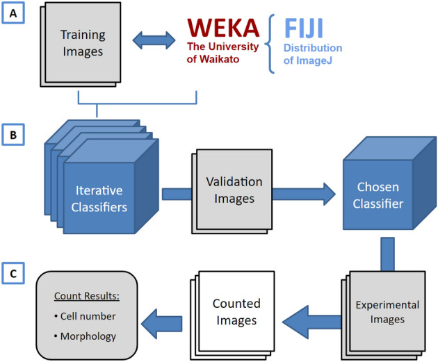
Figure 1 A visual overview of ACCT components and process. (A) Weka and a set of training images are employed to create multiple classifiers through iterative training. (B) These classifiers are then evaluated in bulk against validation images and the best classifier is chosen by the user. (C) The chosen classifier is applied to the experimental dataset for cell quantification, producing a set of counted images and the number of cells in each image, as well as information about the cell morphology. This information includes the area, position, minimum and maximum intensity, circularity, skew, and more details about each cell, available on GitHub in the data availability section.
Figure 1 A visual overview of ACCT components and process. (A) Weka and a set of training images are employed to create multiple classifiers through iterative training. (B) These classifiers are then evaluated in bulk against validation images and the best classifier is chosen by the user. (C) The chosen classifier is applied to the experimental dataset for cell quantification, producing a set of counted images and the number of cells in each image, as well as information about the cell morphology. This information includes the area, position, minimum and maximum intensity, circularity, skew, and more details about each cell, available on GitHub in the data availability section.CC BY · PubMed Central
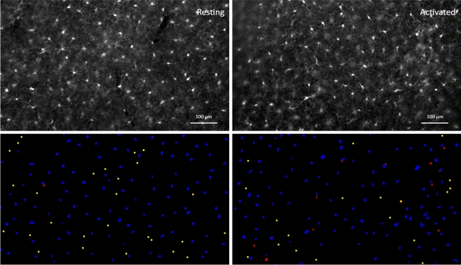
Figure 2 Images of immunofluorescence-labeled microglia before and after segmentation. An example of processed paired images of Iba-1 immunolabeled microglia in cerebral cortex (layer III; Upper panel) of wild-type, non-transgenic (‘Resting’) and of HIVgp120tg mice (‘Activated’), and the accompanying final segmentation images generated via ACCT (lower panel). Resulting object segmentations are color-coded (blue = true positive, red = false positive, yellow = false negative). Segmented objects from images in the same field of view were projected with a size exclusion minimum of 50 pixels for counting. Immunofluorescence staining and acquisition of images are described in previous publications and the Methods Section17. Scale bar: 100 μm.
Figure 2 Images of immunofluorescence-labeled microglia before and after segmentation. An example of processed paired images of Iba-1 immunolabeled microglia in cerebral cortex (layer III; Upper panel) of wild-type, non-transgenic (‘Resting’) and of HIVgp120tg mice (‘Activated’), and the accompanying final segmentation images generated via ACCT (lower panel). Resulting object segmentations are color-coded (blue = true positive, red = false positive, yellow = false negative). Segmented objects from images in the same field of view were projected with a size exclusion minimum of 50 pixels for counting. Immunofluorescence staining and acquisition of images are described in previous publications and the Methods Section17. Scale bar: 100 μm.CC BY · PubMed Central
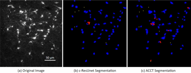
Figure 3 Image of fluorescence-labeled neurons before and after segmentation. A cropped image taken from the Fluocell dataset paired with cell segmentation (a). This depicts segmented cell objects from image MAR38S1C3R1_DMR_20_o reported in the publicly available Fluocell dataset segmented by c-ResUnet10 (b) and ACCT with classifierBayes3 (c). Resulting object segmentations are color-coded (blue = true positive, red = false positive, yellow = false negative). ACCT was set to filter out objects smaller than 250 pixels and greater than 5000 pixels to remove noise. We applied the watershed algorithm to this dataset. ACCT correctly identified 84.6% of the hand counts in this image and c-ResUnet 86.2%, while ACCT was correct with 86.9% of all predictions and c-ResUnet with 93.3%. Scale bar: 50 μm.
Figure 3 Image of fluorescence-labeled neurons before and after segmentation. A cropped image taken from the Fluocell dataset paired with cell segmentation (a). This depicts segmented cell objects from image MAR38S1C3R1_DMR_20_o reported in the publicly available Fluocell dataset segmented by c-ResUnet10 (b) and ACCT with classifierBayes3 (c). Resulting object segmentations are color-coded (blue = true positive, red = false positive, yellow = false negative). ACCT was set to filter out objects smaller than 250 pixels and greater than 5000 pixels to remove noise. We applied the watershed algorithm to this dataset. ACCT correctly identified 84.6% of the hand counts in this image and c-ResUnet 86.2%, while ACCT was correct with 86.9% of all predictions and c-ResUnet with 93.3%. Scale bar: 50 μm.CC BY · PubMed Central
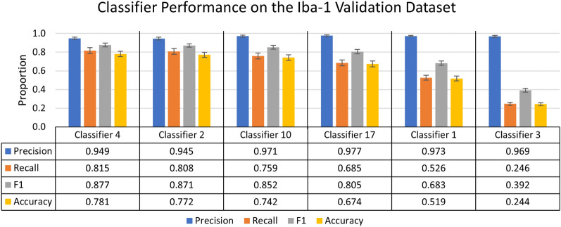
Figure 4 Summary of individual classifier performance on the Iba-1 microglia dataset during the validation stage. A chart of the most and least accurate three incrementally trained classifiers, ranked by F1 score of 25 trained classifiers (n = 10 images). Error bars represent standard error of the mean on calculated performance statistics from each image, where the statistic itself is calculated from total cells in the dataset. The parameters used in ACCT: 0.5 threshold, 50 minimum pixel size, and 1,000 maximum pixel size.
Figure 4 Summary of individual classifier performance on the Iba-1 microglia dataset during the validation stage. A chart of the most and least accurate three incrementally trained classifiers, ranked by F1 score of 25 trained classifiers (n = 10 images). Error bars represent standard error of the mean on calculated performance statistics from each image, where the statistic itself is calculated from total cells in the dataset. The parameters used in ACCT: 0.5 threshold, 50 minimum pixel size, and 1,000 maximum pixel size.CC BY · PubMed Central
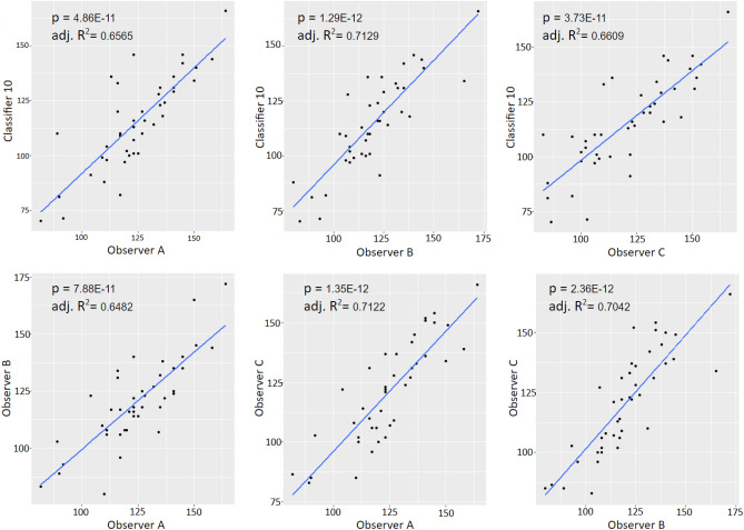
Figure 5 Correlation analysis of microglial density scatter plots with regression lines for all correlative comparisons between observer counts and the automatic count from classifier 10 for the experimental dataset. All relationships showed significant, positive overall correlations (p and Adj. R² = values included in the figures; n=42).
Figure 5 Correlation analysis of microglial density scatter plots with regression lines for all correlative comparisons between observer counts and the automatic count from classifier 10 for the experimental dataset. All relationships showed significant, positive overall correlations (p and Adj. R² = values included in the figures; n=42).CC BY · PubMed Central
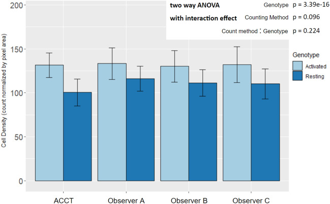
Figure 6 Mean microglia density by experimental genotype in manual and automated counts. All counting methods found an increase in microglia density in Activated microglia images by two way ANOVA with interaction effect and Tukey HSD post-hoc analysis. The difference between counting method and the interaction effect did not display statistical significance. (Genotype: p = 3.39E⁻¹⁶; Counting Method: p = 0.096; Genotype:Counting Method: p = 0.224; Resting n = 22, Activated n = 20). There were not significant differences between the automatic count and Observer B and C. However, the ACCT count density trended lower overall than Observer A’s (p = 0.0599; Resting n = 22, Activated n = 20). This suggests that classifier 10 may have excluded some faintly stained or not well-in-focus cells in the Resting group images that Observer A did count. Error bars represent standard deviation.
Figure 6 Mean microglia density by experimental genotype in manual and automated counts. All counting methods found an increase in microglia density in Activated microglia images by two way ANOVA with interaction effect and Tukey HSD post-hoc analysis. The difference between counting method and the interaction effect did not display statistical significance. (Genotype: p = 3.39E⁻¹⁶; Counting Method: p = 0.096; Genotype:Counting Method: p = 0.224; Resting n = 22, Activated n = 20). There were not significant differences between the automatic count and Observer B and C. However, the ACCT count density trended lower overall than Observer A’s (p = 0.0599; Resting n = 22, Activated n = 20). This suggests that classifier 10 may have excluded some faintly stained or not well-in-focus cells in the Resting group images that Observer A did count. Error bars represent standard deviation.CC BY · PubMed Central
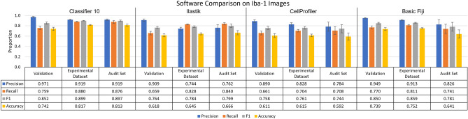
Figure 7 ACCT vs Ilastik vs CellProfiler vs Basic Fiji on images of Iba-1 positive microglia. The performance of ACCT classifier 10 versus Ilastik, CellProfiler, and basic use of Fiji tools. The audit set is a selection of 10 images, which is equal to the size of the validation image set, chosen from the experimental dataset and evenly distributed between experimental groups. Error bars represent standard error of the mean on calculated performance statistics from each image, where the statistic itself is calculated from total cells in the dataset. The parameters used by ACCT in this analysis were: a 0.5 threshold, 50 minimum pixel size, 1,000 maximum pixel size for objects.
Figure 7 ACCT vs Ilastik vs CellProfiler vs Basic Fiji on images of Iba-1 positive microglia. The performance of ACCT classifier 10 versus Ilastik, CellProfiler, and basic use of Fiji tools. The audit set is a selection of 10 images, which is equal to the size of the validation image set, chosen from the experimental dataset and evenly distributed between experimental groups. Error bars represent standard error of the mean on calculated performance statistics from each image, where the statistic itself is calculated from total cells in the dataset. The parameters used by ACCT in this analysis were: a 0.5 threshold, 50 minimum pixel size, 1,000 maximum pixel size for objects.CC BY · PubMed Central
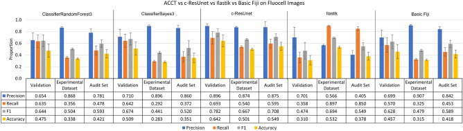
Figure 8 ACCT vs c-ResUnet vs Ilastik vs Basic Fiji on the Fluocell dataset. ClassifierRandomForest3 and ClassifierBayes3 are the third trained iterations of a Fast Random Forest and BayesNet model in ACCT, respectively. The three tools’ automatic counts of the Fluocell images and basic use of Fiji tools are compared to our manual count of the Fluocell dataset. Error bars represent standard error of the mean on calculated performance statistics from each image, where the statistic itself is calculated from total cells in the dataset. The audit set is a selection of 10 images, which is equal to the size of the validation image set, chosen from the experimental dataset. The parameters used are: a 0.5 threshold, 250 minimum pixel size, 5000 maximum pixel size, and with the watershed algorithm applied.
Figure 8 ACCT vs c-ResUnet vs Ilastik vs Basic Fiji on the Fluocell dataset. ClassifierRandomForest3 and ClassifierBayes3 are the third trained iterations of a Fast Random Forest and BayesNet model in ACCT, respectively. The three tools’ automatic counts of the Fluocell images and basic use of Fiji tools are compared to our manual count of the Fluocell dataset. Error bars represent standard error of the mean on calculated performance statistics from each image, where the statistic itself is calculated from total cells in the dataset. The audit set is a selection of 10 images, which is equal to the size of the validation image set, chosen from the experimental dataset. The parameters used are: a 0.5 threshold, 250 minimum pixel size, 5000 maximum pixel size, and with the watershed algorithm applied.CC BY · PubMed Central
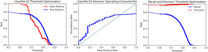
Figure 9 An ROC curve generated by ACCT following the validation stage on Iba-1 microglia images. It depicts the false positive, true positive, recall, and precision rates of classifier 10 at different confidence thresholds on the Iba-1 stained microglia images. Objects were filtered to a minimum size of 50 pixels and a maximum size of 1000 pixels. The watershed algorithm was not applied to the Iba-1 dataset, due to consistent cell separation in the sample tissues.
Figure 9 An ROC curve generated by ACCT following the validation stage on Iba-1 microglia images. It depicts the false positive, true positive, recall, and precision rates of classifier 10 at different confidence thresholds on the Iba-1 stained microglia images. Objects were filtered to a minimum size of 50 pixels and a maximum size of 1000 pixels. The watershed algorithm was not applied to the Iba-1 dataset, due to consistent cell separation in the sample tissues.CC BY · PubMed Central

Verification

Claims the paper makes

The claims and statistics of this paper haven’t been checked yet.

Run the check — free, no account needed. It reads the open-access text and checks the sources it cites.

A few free checks a day · papers already verified open instantly · results are public

Claims other papers make about this one

Each is checked against this paper’s own text: does it say what the citing paper says it does?

Self-check

Percentages, sums and reported differences re-computed from the paper’s own numbers.

The self-check needs the paper’s full text.

Citations

Cites

Show all 3 references

Research works printed but not linked: 23

  1. Jensen, E. C. Quantitative analysis of histological staining and fluorescence using ImageJ. Am. Assoc. Anat. 296, 378–381. https://doi.org/10.1002/ar.22641 (2013). · DOI
  2. Schneider, C. A., Rasband, W. S. & Eliceiri, K. W. Nih image to imagej: 25 years of image analysis. Nat. Methods 9, 671–675. https://doi.org/10.1038/nmeth.2089 (2012). · DOI · Paper page
  3. Arganda-Carreras, I. et al. Trainable Weka Segmentation: A machine learning tool for microscopy pixel classification. Bioinformatics 33, 2424–2426. https://doi.org/10.1093/bioinformatics/btx180 (2017). · DOI · Paper page
  4. Toggas, S. M. et al. Central nervous system damage produced by expression of the hiv-1 coat protein gpl20 in transgenic mice. Nature 367, 188–193. https://doi.org/10.1038/367188a0 (1994). · DOI
  5. Lynch, M. A. The multifaceted profile of activated microglia. Mol. Neurobiol. 40, 139–156. https://doi.org/10.1007/s12035-009-8077-9 (2009). · DOI · Paper page
  6. Karperien, A., Ahammer, H. & Jelinek, H. Quantitating the subtleties of microglial morphology with fractal analysis. Front. Cell. Neurosci. 7, 3. https://doi.org/10.3389/fncel.2013.00003 (2013). · DOI
  7. Morelli, R. et al. Automating cell counting in fluorescent microscopy through deep learning with c-resunet. Sci. Rep. 11, 1–11. https://doi.org/10.1038/s41598-021-01929-5 (2021). · DOI
  8. Goecks, J., Nekrutenko, A. & Taylor, J. Galaxy: A comprehensive approach for supporting accessible, reproducible, and transparent computational research in the life sciences. Genome Biol. 11, 1–13. https://doi.org/10.1186/gb-2010-11-8-r86 (2010). · DOI
  9. Berg, S. et al. Ilastik: interactive machine learning for (bio) image analysis. Nat. Methods 16, 1226–1232. https://doi.org/10.1038/s41592-019-0582-9 (2019). · DOI
  10. Diakogiannis, F. I., Waldner, F., Caccetta, P. & Wu, C. Resunet-a: A deep learning framework for semantic segmentation of remotely sensed data. ISPRS Journal of Photogrammetry and Remote Sensing 162, 94–114. https://doi.org/10.1016/j.isprsjprs.2020.01.013 (2020). · DOI
  11. Stirling, D. R. et al. Cellprofiler 4: Improvements in speed, utility and usability. BMC Bioinform. 22, 1–11. https://doi.org/10.1186/s12859-021-04344-9 (2021). · DOI
  12. Dao, D. et al. Cellprofiler analyst: Interactive data exploration, analysis and classification of large biological image sets. Bioinformatics 32, 3210–3212. https://doi.org/10.1093/bioinformatics/btw390 (2016). · DOI
  13. Singh, H. et al. A pivotal role for interferon-$$\alpha$$ receptor-1 in neuronal injury induced by hiv-1. J. Neuroinflamm. 17, 226. https://doi.org/10.1186/s12974-020-01894-2 (2020). · DOI
  14. Schindelin, J. et al. Fiji: An open-source platform for biological-image analysis. Nat. Methods 9, 676–682. https://doi.org/10.1038/nmeth.2019 (2012). · DOI · Paper page
  15. Virtanen, P. et al. SciPy 1.0: Fundamental algorithms for scientific computing in Python. Nat. Methods 17, 261–272. https://doi.org/10.1038/s41592-019-0686-2 (2020). · DOI · Paper page
  16. McKinney, W. et al. Data structures for statistical computing in python. In Proceedings of the 9th Python in Science Conference vol. 445, 51–56 (2010). · DOI
  17. Harris, C. R. et al. Array programming with NumPy. Nature 585, 357–362. https://doi.org/10.1038/s41586-020-2649-2 (2020). · DOI · Paper page
  18. Hunter, J. D. Matplotlib: A 2d graphics environment. Comput. Sci. Eng. 9, 90–95 (2007). · DOI · Paper page
  19. Pedregosa, F. et al. Scikit-learn: Machine learning in python. J. Mach. Learn. Res. 12, 2825–2830. https://doi.org/10.5555/1953048.2078195 (2011). · DOI
  20. Breiman, L. Random forests. Mach. Learn. 45, 5–32. https://doi.org/10.1023/A:1010933404324 (2001). · DOI · Paper page
  21. Friedman, N., Geiger, D. & Goldszmidt, M. Bayesian network classifiers. Mach. Learn. 29, 131–163. https://doi.org/10.1023/A:1007465528199 (1997). · DOI · Paper page
  22. Vincent, L. & Soille, P. Watersheds in digital spaces: An efficient algorithm based on immersion simulations. IEEE Trans. Pattern Anal. Mach. Intell. 13, 583–598. https://doi.org/10.1109/34.87344 (1991). · DOI
  23. Yan, Q., Zheng, J., Reding, S., Li, S. & Doytchinov, I. Crossloc: Scalable aerial localization assisted by multimodal synthetic data. In Proceedings of the IEEE/CVF Conference on Computer Vision and Pattern Recognition 17358–17368, https://doi.org/10.48550/arXiv.2112.09081(2022). · DOI

Cited by

Sorted by citations

Metadata

Authors
Kataras, T. J., Jang, T. J., Koury, J., Singh, H., Fok, D., & Kaul, M.
Venue
Scientific Reports
Published
2023-05-22
Volume
13
Issue
1
ISSN
2045-2322
Cited by
26
References
3
Language
en
Funders
National Institutes of Health (R01 MH104131)

About these checks

Registry, retraction, Cites and statistics results are computed, not judged, with one exception: a printed reference that no index lists is read once by a model before it counts as a citation error. Claims are extracted by a model and kept only when their quote appears verbatim in the text; each cited source is then checked, with a model’s help, for whether it says what the claim relies on. Those verdicts can be wrong — read the claim’s quote and the cited source before relying on one.

Statistics and arithmetic are recomputed, not judged.

Confidence bands are shown only for fields calibrated on our annotated test set. None is calibrated yet, so no band is shown.

What counts as a claim ›How we measure confidence ›How we check this ›

Are you an author, or do you see a problem with this page? Request a review