Cited by 104Visual perception and processing mechanismsNeural dynamics and brain functionFace Recognition and Perception

The DOI matches its Crossref record; 58 of the 59 references it cites were found in a registry or an index.

Activations of deep convolutional neural networks are aligned with gamma band activity of human visual cortex

Open access

Published version of a preprint

Abstract

Recent advances in the field of artificial intelligence have revealed principles about neural processing, in particular about vision. Previous work demonstrated a direct correspondence between the hierarchy of the human visual areas and layers of deep convolutional neural networks (DCNN) trained on visual object recognition. We use DCNN to investigate which frequency bands correlate with feature transformations of increasing complexity along the ventral visual pathway. By capitalizing on intracranial depth recordings from 100 patients we assess the alignment between the DCNN and signals at different frequency bands. We find that gamma activity (30–70 Hz) matches the increasing complexity of visual feature representations in DCNN. These findings show that the activity of the DCNN captures the essential characteristics of biological object recognition not only in space and time, but also in the frequency domain. These results demonstrate the potential that artificial intelligence algorithms have in advancing our understanding of the brain.

Overview

The claims and statistics of this paper haven’t been checked yet.

Run the check — free, no account needed. It reads the open-access text and checks the sources it cites.

A few free checks a day · papers already verified open instantly · results are public

Integrity signals

Registry

Crossref · 10.1038/s42003-018-0110-y

Cites

58 of 58 references verified0 citation errors · 0 not checkable

Statistics

Figures

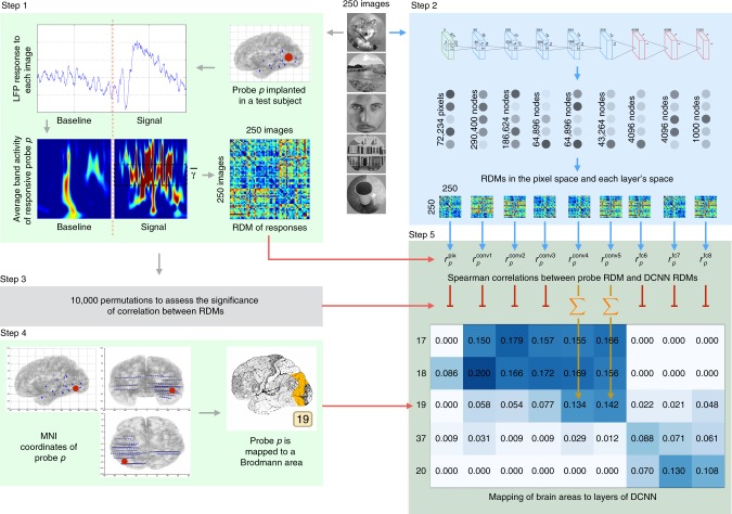
Fig. 1 Overview of the analysis pipeline. Two hundred and fifty natural images are presented to human subjects (Step 1) and to an artificial vision system (Step 2). The activities elicited in these two systems are compared in order to map regions of human visual cortex to layers of deep convolutional neural networks (DCNNs). Step 1: LFP response of each of 11,293 electrodes to each of the images is converted into the frequency domain. Activity evoked by each image is compared to the activity evoked by every other image and results of this comparison are presented as a representational dissimilarity matrix (RDM). Step 2: Each of the images is shown to a pretrained DCNN and activations of each of the layers are extracted. Each layer’s activations form a representation space, in which stimuli (images) can be compared to each other. Results of this comparison are summarized as a RDM for each DCNN layer. Step 3: Subject’s intracranial responses to stimuli are randomly reshuffled and the analysis performed in step 1 is repeated 10,000 times to obtain 10,000 random RDMs for each electrode. Step 4: Each electrode’s MNI coordinates are used to map the electrode to a Brodmann area. The figure also gives an example of electrode implantation locations in one of the subjects (blue circles are the electrodes). Step 5: Spearman’s rank correlation is computed between the true (nonpermuted) RDM of neural responses and RDMs of each layer of DCNN. Also 10,000 scores are computed with the random RDM for each electrode-layer pair to assess the significance of the true correlation score. If the score obtained with the true RDM is significant (the value of p < 0.001 is estimated by selecting a threshold such that none of the probes would pass it on the permuted data), then the score is added to the mapping matrix. The procedure is repeated for each electrode and the correlation scores are summed and normalized by the number of electrodes per Brodmann area. The resulting mapping matrix shows the alignment between the consecutive areas of the ventral stream and layers of DCNN
Fig. 1 Overview of the analysis pipeline. Two hundred and fifty natural images are presented to human subjects (Step 1) and to an artificial vision system (Step 2). The activities elicited in these two systems are compared in order to map regions of human visual cortex to layers of deep convolutional neural networks (DCNNs). Step 1: LFP response of each of 11,293 electrodes to each of the images is converted into the frequency domain. Activity evoked by each image is compared to the activity evoked by every other image and results of this comparison are presented as a representational dissimilarity matrix (RDM). Step 2: Each of the images is shown to a pretrained DCNN and activations of each of the layers are extracted. Each layer’s activations form a representation space, in which stimuli (images) can be compared to each other. Results of this comparison are summarized as a RDM for each DCNN layer. Step 3: Subject’s intracranial responses to stimuli are randomly reshuffled and the analysis performed in step 1 is repeated 10,000 times to obtain 10,000 random RDMs for each electrode. Step 4: Each electrode’s MNI coordinates are used to map the electrode to a Brodmann area. The figure also gives an example of electrode implantation locations in one of the subjects (blue circles are the electrodes). Step 5: Spearman’s rank correlation is computed between the true (nonpermuted) RDM of neural responses and RDMs of each layer of DCNN. Also 10,000 scores are computed with the random RDM for each electrode-layer pair to assess the significance of the true correlation score. If the score obtained with the true RDM is significant (the value of p < 0.001 is estimated by selecting a threshold such that none of the probes would pass it on the permuted data), then the score is added to the mapping matrix. The procedure is repeated for each electrode and the correlation scores are summed and normalized by the number of electrodes per Brodmann area. The resulting mapping matrix shows the alignment between the consecutive areas of the ventral stream and layers of DCNNCC BY · PubMed Central
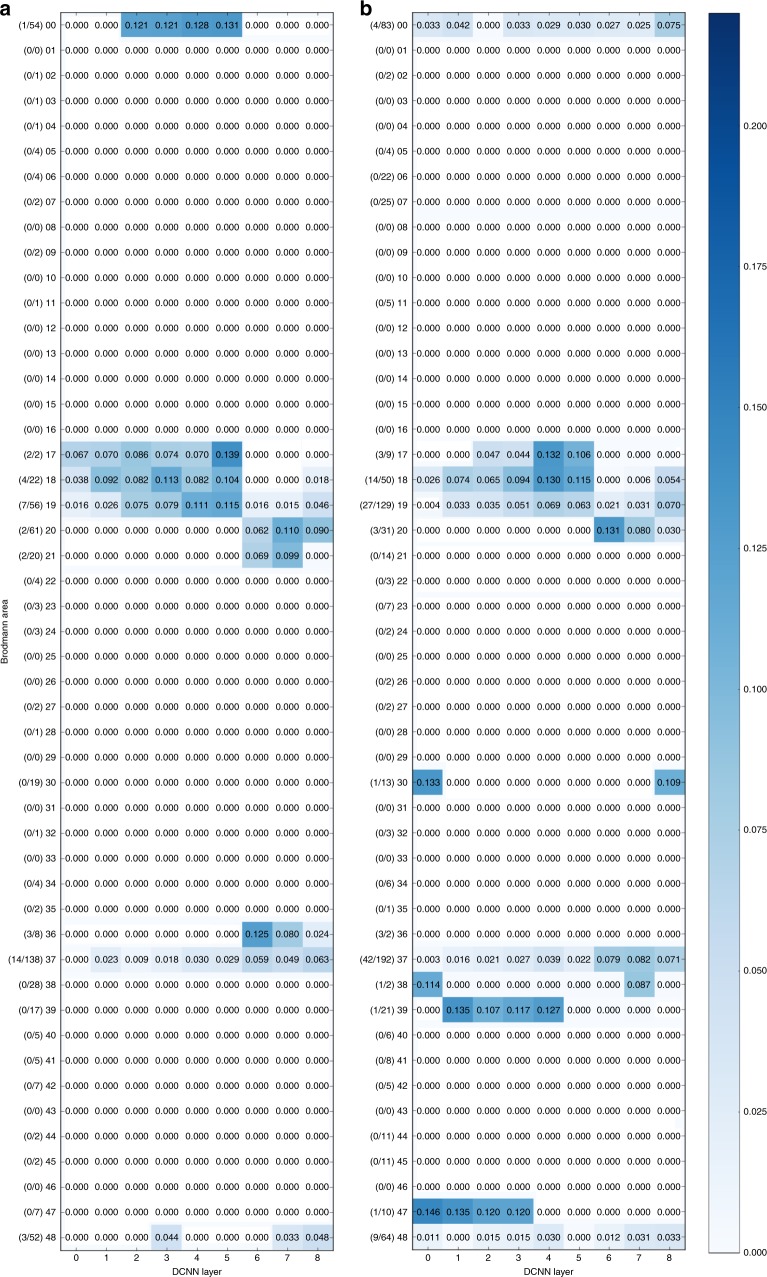
Fig. 2 Mapping of the activity in Brodmann areas to DCNN layers. Underlying data comes from the activity in low gamma (31–70 Hz, a) and high-gamma (71–150 Hz, b) bands in 150–350 ms time window. On the vertical axis there are Brodmann areas and the number of significantly correlating probes in each area out of the total number of responsive probes in that area. Horizontal axis represents succession of layers of DCNN. Number in each cell of the matrix is the total sum of correlations (between RDMs of probes in that particular area and the RDM of that layer) normalized by the number of significantly correlating probes in an area
Fig. 2 Mapping of the activity in Brodmann areas to DCNN layers. Underlying data comes from the activity in low gamma (31–70 Hz, a) and high-gamma (71–150 Hz, b) bands in 150–350 ms time window. On the vertical axis there are Brodmann areas and the number of significantly correlating probes in each area out of the total number of responsive probes in that area. Horizontal axis represents succession of layers of DCNN. Number in each cell of the matrix is the total sum of correlations (between RDMs of probes in that particular area and the RDM of that layer) normalized by the number of significantly correlating probes in an areaCC BY · PubMed Central
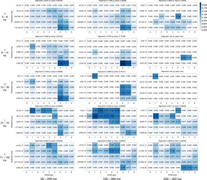
Fig. 3 Mapping of activity in visual areas to activations of layers of DCNN across five frequency bands and three time windows. Vertical axis holds Brodmann areas in the order of the ventral stream (top to bottom), horizontal axis represents the succession of layers of DCNN. Number in each cell of a matrix is the total sum of correlations (between RDMs of probes in that particular area and the RDM of that layer) normalized by the number of significantly correlating probes in an area. The alignment score is computed as Spearman’s rank correlation between electrode assignment to Brodmann areas and electrode assignment to DCNN layers (Eq. (8)). The numbers on the left of each subplot show the number of significantly correlating probes in each area out of the total number of responsive probes in that area
Fig. 3 Mapping of activity in visual areas to activations of layers of DCNN across five frequency bands and three time windows. Vertical axis holds Brodmann areas in the order of the ventral stream (top to bottom), horizontal axis represents the succession of layers of DCNN. Number in each cell of a matrix is the total sum of correlations (between RDMs of probes in that particular area and the RDM of that layer) normalized by the number of significantly correlating probes in an area. The alignment score is computed as Spearman’s rank correlation between electrode assignment to Brodmann areas and electrode assignment to DCNN layers (Eq. (8)). The numbers on the left of each subplot show the number of significantly correlating probes in each area out of the total number of responsive probes in that areaCC BY · PubMed Central
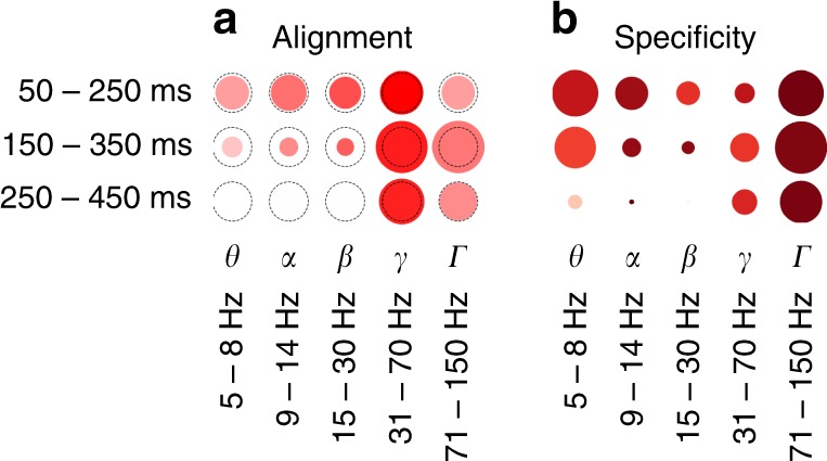
Fig. 4 Overall relative statistics of brain responses across frequency bands and time windows. a The alignment between visual brain areas and DCNN layers (see Eq. (8)). The color indicates the correlation value (ρ) while the size of the marker shows the logarithm (so that not significant results are still visible on the plot) of inverse of the statistical significance of the correlation, dotted circle indicates p = 0.0003(3)—the Bonferroni-corrected significance threshold level of 0.005. b Activity in a region of interest is specific to visual areas (see Eq. (4)): intense red means that most of the activity in that band and time window happened in visual areas, size of the marker indicates total volume (Eq. (2)) of activity in all areas. The maximal size of a marker is defined by the biggest marker on the figure
Fig. 4 Overall relative statistics of brain responses across frequency bands and time windows. a The alignment between visual brain areas and DCNN layers (see Eq. (8)). The color indicates the correlation value (ρ) while the size of the marker shows the logarithm (so that not significant results are still visible on the plot) of inverse of the statistical significance of the correlation, dotted circle indicates p = 0.0003(3)—the Bonferroni-corrected significance threshold level of 0.005. b Activity in a region of interest is specific to visual areas (see Eq. (4)): intense red means that most of the activity in that band and time window happened in visual areas, size of the marker indicates total volume (Eq. (2)) of activity in all areas. The maximal size of a marker is defined by the biggest marker on the figureCC BY · PubMed Central
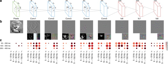
Fig. 5 Specificity of neural responses to layers of DCNN across frequency bands and time windows. a The architecture of the DCNN. Convolutional layer 1 consists of 96 feature detectors of size 11 × 11, they take as input pixels of the image and their activations create 96 features maps of size 55 × 55, architecture of all consecutive convolutional layers is analogous. Five convolutional layers are followed by three fully connected layers of sizes 4096, 4096, and 1000, respectively. b The leftmost image is an example input image. For each layer we have selected one interesting filter that depicts what is happening inside of the neural network and plotted: (a) a reconstruction of the original image from the activity of that neuron using the deconvolution48 technique (upper larger image), (b) activations on the feature map generated by that neuron (left subimage), and (c) synthetic image that shows what input the neuron would be most responsive to (right subimage). Visualizations were made with Deep Visualization Toolbox55. All filters are canonical to AlexNet trained on ImageNet and can be explored using the above-mentioned visualization tool or visualized directly from the publicly available weights of the network. c Specificity of neural responses across frequency bands and time windows for each layer of DCNN. Size of a marker is the total activity mapped to this layer and the intensity of the color is the specificity of the activity to the Brodmann areas constituting the ventral stream: BA17-18-19-37-20
Fig. 5 Specificity of neural responses to layers of DCNN across frequency bands and time windows. a The architecture of the DCNN. Convolutional layer 1 consists of 96 feature detectors of size 11 × 11, they take as input pixels of the image and their activations create 96 features maps of size 55 × 55, architecture of all consecutive convolutional layers is analogous. Five convolutional layers are followed by three fully connected layers of sizes 4096, 4096, and 1000, respectively. b The leftmost image is an example input image. For each layer we have selected one interesting filter that depicts what is happening inside of the neural network and plotted: (a) a reconstruction of the original image from the activity of that neuron using the deconvolution48 technique (upper larger image), (b) activations on the feature map generated by that neuron (left subimage), and (c) synthetic image that shows what input the neuron would be most responsive to (right subimage). Visualizations were made with Deep Visualization Toolbox55. All filters are canonical to AlexNet trained on ImageNet and can be explored using the above-mentioned visualization tool or visualized directly from the publicly available weights of the network. c Specificity of neural responses across frequency bands and time windows for each layer of DCNN. Size of a marker is the total activity mapped to this layer and the intensity of the color is the specificity of the activity to the Brodmann areas constituting the ventral stream: BA17-18-19-37-20CC BY · PubMed Central
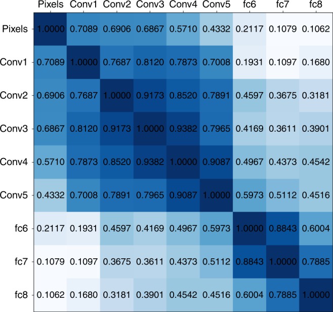
Fig. 6 Correlations between the representation dissimilarity matrices of the layers of the deep convolutional neural network. All scores are significant
Fig. 6 Correlations between the representation dissimilarity matrices of the layers of the deep convolutional neural network. All scores are significantCC BY · PubMed Central
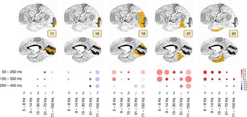
Fig. 7 Area-specific analysis of volume of neural activity and complexity of visual features represented by that activity. Size of the marker shows the sum of correlation coefficients between the area and DCNN for each particular band and time window. Color codes the ratio of complex visual features to simple visual features, i.e., the comparison between the activity that correlates with the higher layers (conv5, fc6, and fc7) of DCNN to the lower layers (conv1, conv2, and conv3). Intense red means that the activity was correlating more with the activity of higher layers of DCNN, while the intense blue indicates the dominance of correlation with the lower areas. If the color is close to white then the activations of both lower and higher layers of DCNN were correlating with the brain responses in approximately equal proportion
Fig. 7 Area-specific analysis of volume of neural activity and complexity of visual features represented by that activity. Size of the marker shows the sum of correlation coefficients between the area and DCNN for each particular band and time window. Color codes the ratio of complex visual features to simple visual features, i.e., the comparison between the activity that correlates with the higher layers (conv5, fc6, and fc7) of DCNN to the lower layers (conv1, conv2, and conv3). Intense red means that the activity was correlating more with the activity of higher layers of DCNN, while the intense blue indicates the dominance of correlation with the lower areas. If the color is close to white then the activations of both lower and higher layers of DCNN were correlating with the brain responses in approximately equal proportionCC BY · PubMed Central

Verification

Claims the paper makes

The claims and statistics of this paper haven’t been checked yet.

Run the check — free, no account needed. It reads the open-access text and checks the sources it cites.

A few free checks a day · papers already verified open instantly · results are public

Claims other papers make about this one

Each is checked against this paper’s own text: does it say what the citing paper says it does?

Self-check

Percentages, sums and reported differences re-computed from the paper’s own numbers.

The self-check needs the paper’s full text.

Citations

Cites

Show all 59 references

Research works printed but not linked: 1

  1. Seeliger, K. et al. CNN-based encoding and decoding of visual object recognition in space and time. bioRxiv https://doi.org/10.1101/118091 (2017). · DOI

Cited by

Sorted by citations

Items 101–104 of 104

Metadata

Authors
Kuzovkin, I., Vicente, R., Petton, M., Lachaux, J.-P., Baciu, M., Kahane, P., Rheims, S., Vidal, J. R., & Aru, J.
Affiliations
  • University of Tartu (EE)
  • Lyon 1 Université (FR)
  • Centre National de la Recherche Scientifique (FR)
  • Inserm (FR)
  • Université catholique de lyon (FR)
Corresponding author
  • Kuzovkin, Ilya
  • Aru, Jaan
Venue
Communications Biology
Published
2018-08-08
Volume
1
Issue
1
Pages
107-107
ISSN
2399-3642 (ISSN-L)
OpenAlex
W2949411980
Cited by
104
References
59
Citations by year
2026: 2 · 2025: 17 · 2024: 14 · 2023: 16 · 2022: 13 · 2021: 14 · 2020: 14 · 2019: 7 · 2018: 7
FWCI
6.25
Type
journal article
Language
en
Open access
Locations
  • Communications Biology (publishedVersion, cc-by)
  • bioRxiv (Cold Spring Harbor Laboratory) (acceptedVersion, cc-by)
  • Europe PMC (PubMed Central) (publishedVersion, cc-by)
  • PubMed Central (publishedVersion, cc-by)
  • PubMed (publishedVersion)
  • HAL (submittedVersion, other-oa)
  • DOAJ (DOAJ: Directory of Open Access Journals) (submittedVersion)
Funders
Eesti Teadusagentuur (PUT438, PUT1476)
Topics
  • Life Sciences › Neuroscience › Cognitive Neuroscience › Visual perception and processing mechanisms
  • Life Sciences › Neuroscience › Cognitive Neuroscience › Neural dynamics and brain function
  • Life Sciences › Neuroscience › Cognitive Neuroscience › Face Recognition and Perception
Keywords
deep convolutional neural networks, gamma oscillations, visual cortex, ventral stream, visual feature representation, object recognition

About these checks

Registry, retraction, Cites and statistics results are computed, not judged, with one exception: a printed reference that no index lists is read once by a model before it counts as a citation error. Claims are extracted by a model and kept only when their quote appears verbatim in the text; each cited source is then checked, with a model’s help, for whether it says what the claim relies on. Those verdicts can be wrong — read the claim’s quote and the cited source before relying on one.

Statistics and arithmetic are recomputed, not judged.

Confidence bands are shown only for fields calibrated on our annotated test set. None is calibrated yet, so no band is shown.

What counts as a claim ›How we measure confidence ›How we check this ›

Are you an author, or do you see a problem with this page? Request a review