

The DOI matches its Crossref record; 56 of the 57 references it cites were found in a registry or an index; 16 of the 29 sources its claims cite were checked for support.
A statistical framework for high-content phenotypic profiling using cellular feature distributions
Open accessAbstract
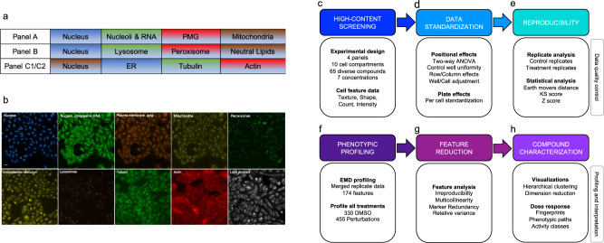
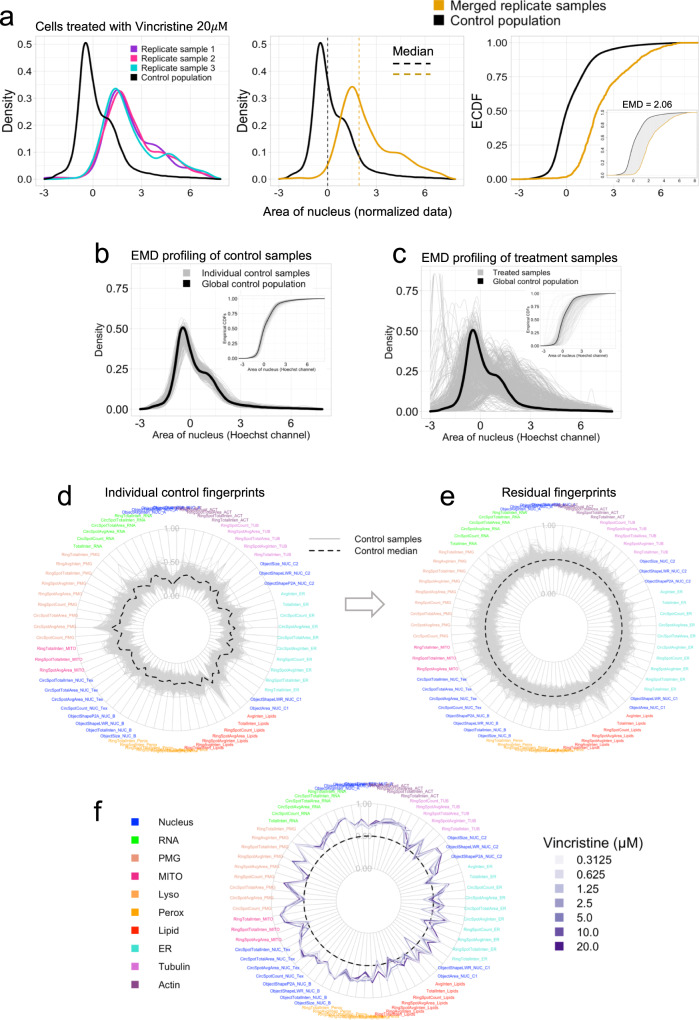
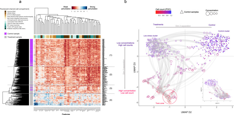
High-content screening (HCS) uses microscopy images to generate phenotypic profiles of cell morphological data in high-dimensional feature space. While HCS provides detailed cytological information at single-cell resolution, these complex datasets are usually aggregated into summary statistics that do not leverage patterns of biological variability within cell populations. Here we present a broad-spectrum HCS analysis system that measures image-based cell features from 10 cellular compartments across multiple assay panels. We introduce quality control measures and statistical strategies to streamline and harmonize the data analysis workflow, including positional and plate effect detection, biological replicates analysis and feature reduction. We also demonstrate that the Wasserstein distance metric is superior over other measures to detect differences between cell feature distributions. With this workflow, we define per-dose phenotypic fingerprints for 65 mechanistically diverse compounds, provide phenotypic path visualizations for each compound and classify compounds into different activity groups.
Overview
CoChat Summary
TL;DR
The paper presents a broad-spectrum high-content screening (HCS) assay and statistical workflow that uses cell-level feature distributions rather than well-averaged summaries to profile phenotypic responses. It reports that the Wasserstein/earth mover’s distance (EMD) is more sensitive than Z-score or Kolmogorov–Smirnov metrics for detecting differences between cell feature distributions and uses the workflow to classify 65 compounds into activity groups.
Key findings
- The assay labels ten cellular compartments across four panels and extracts 174 texture, shape, count, and intensity features; feature reduction removes 60% of features, leaving 69 active features.
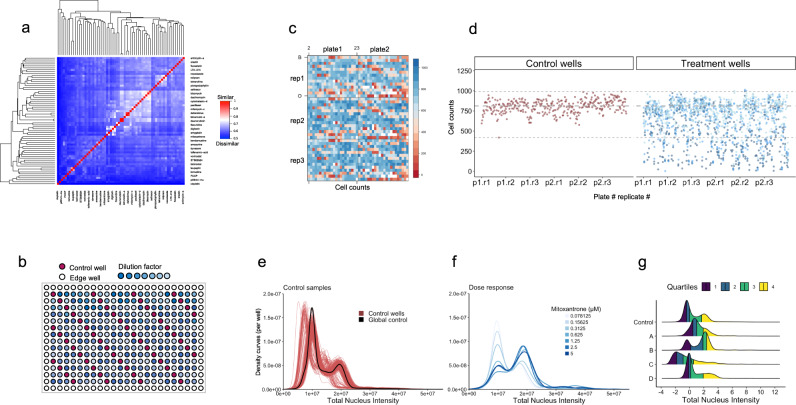
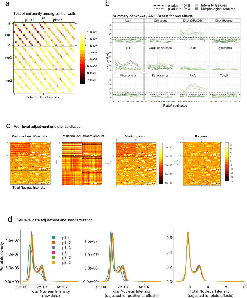
- Positional effects were common for intensity features: 45% of intensity-related features showed significant row or column dependency (P < 0.0001), versus only 6% of morphological features and cell counts.
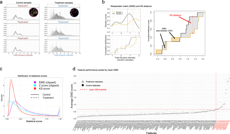
- EMD outperformed Z-score and KS metrics for detecting replicate dissimilarity and distribution differences; it was used to profile 65 compounds at seven concentrations with three technical replicates, using 330 control wells and 455 treatment wells.
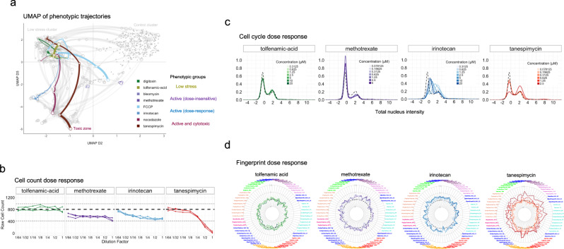
- Phenotypic profiling separated treatments into four broad groups—control, “low stress,” active phenotypes, and broad cytotoxic responses—and showed dose-dependent trajectories; for example, methotrexate reduced cell counts by ~25% and induced G1 arrest, while tanespimycin caused G2/M arrest at 2.5 μM.
Methods
- U2OS cells were seeded in 384-well plates at 1,800 cells/well; 65 diverse compounds were tested at seven concentrations with three technical replicates, alongside 55 DMSO control wells placed in a diagonal pattern. Four staining panels labeled DNA, RNA, mitochondria, plasma membrane/Golgi, lysosomes, peroxisomes, lipid droplets, ER, actin, and tubulin.
- Images were acquired on a Cellomics ArrayScan XTI with a ×20 objective, nine fields per well; 174 features were extracted using Cellomics Compartmental Analysis.
- Analysis included two-way ANOVA for row/column positional effects, median polish adjustment, B-score and per-cell BZ standardization to per-plate controls, comparison of Z-score, KS, and EMD metrics, replicate merging, EMD profiling against a global control, feature reduction, hierarchical clustering, and UMAP; analyses used R and ggplot2.
Limitations
- The paper states that EMD does not take directional changes into account, and that extending it to account for direction could improve downstream profile similarity analysis.
- The paper states that the dataset is not ideal for compound similarity or MOA classification because the 65 compounds were chosen to be diverse with low structural similarity; it also notes that no community-wide consensus or standard HCS workflow exists, limiting cross-study comparison and data integration.
- Evident from the text: the study uses a single cell line (U2OS) and a 24 h treatment period, and some features—especially lysosomal, lipid, and RNA puncta features—were irreproducible or removed due to weak signal, bleed-through, or low biological relevance, which may limit generalizability.
Model-written summary. Check it against the paper before relying on it.
Integrity signals
Registry
Cites
Statistics
Figures
Verification
Claims the paper makes
10 Valid · 3 Not valid · 7 Not checked · 110 Own results and interpretations
The cited sources support only part of this claim — read each source’s verdict below.
In the paper
“In contrast, positional effects due to technical variability manifest as distinct spatial patterns across the rows, columns and edges in different plates, a common challenge in multi-well-based assays30–33.”
§ A statistical framework for high-content phenotypic profiling using cellular feature distributions > Results > Positional effects adjustment and data standardization
What the sources say
- Not checked — no full text of the sourcecites [30] Malo, N., Hanley, J. A., Cerquozzi, S., Pelletier, J. & Nadon, R. Statistical practice in high-throughput screening data analysis. Nat. Biotechnol. 24, 167–175 (2006). source
- Partly supportedcites [31] Yu, H. et al. Positional artifacts in microarrays: experimental verification and construction of COP, an automated detection tool. Nucleic Acids Res. 35, e8 (2007). sourceExperimental — accuracy not yet measured
In Results and Discussion, “Artifact related to positions on microtiter plates” (page unavailable), the paper reports artificially higher correlations among nearby plate positions, linked to cross-contamination, and notes an effect along the Y-direction. It does not describe distinct patterns across rows, columns, and edges of different plates. (LLM, conf=0.84)
- Supportedcites [32] Makarenkov, V. et al. An efficient method for the detection and elimination of systematic error in high-throughput screening. Bioinformatics 23, 1648–1657 (2007). source
The Introduction (page unavailable) says systematic errors create border, row, and column effects in high-throughput screening plates. The Simulation study (page unavailable) also considers positional errors that change from plate to plate, supporting the claim that their patterns can differ across plates. (LLM, conf=0.90)
- Partly supportedcites [33] Homouz, D., Chen, G. & Kudlicki, A. S. Correcting positional correlations in Affymetrix® Genome Chips. Sci. Rep. 5, 9078 (2015). sourceExperimental — accuracy not yet measured
The Results (Evidence of positional artifact; page unavailable) describe a spatial, distance-dependent correlation pattern on Affymetrix chips that the authors propose arises from experimental systematic errors. The Discussion says the artifact varies across chip platforms. The paper does not establish row, column, or edge patterns in multi-well plates; it also attributes one prominent x-axis pattern to the arrangement of genes on the chip rather than technical variability. (LLM, conf=0.87)
plainstates a cause- Asserted: passes — The authors put it forward as true.
- Checkable: passes — It can be checked against evidence.
- Load-bearing: passes — The paper’s conclusions depend on it.
- Based: passes — The paper gives a reason why it holds.
The cited sources support only part of this claim — read each source’s verdict below.
In the paper
“First, positional effects (edge effects, row/column dependencies, or gradient artifacts) are a persistent factor in multi-well assays and microarray experiments30,31,52.”
§ A statistical framework for high-content phenotypic profiling using cellular feature distributions > Discussion
What the sources say
- Not checked — no full text of the sourcecites [30] Malo, N., Hanley, J. A., Cerquozzi, S., Pelletier, J. & Nadon, R. Statistical practice in high-throughput screening data analysis. Nat. Biotechnol. 24, 167–175 (2006). source
- Partly supportedcites [31] Yu, H. et al. Positional artifacts in microarrays: experimental verification and construction of COP, an automated detection tool. Nucleic Acids Res. 35, e8 (2007). sourceExperimental — accuracy not yet measured
The Results and Discussion sections on plate artifacts and their consequences report positional artifacts in every microarray experiment examined, including effects associated with locations on microtiter plates. The paper does not establish that these effects persist across multi-well assays generally, or specifically document edge effects and gradient artifacts. (LLM, conf=0.85)
- Partly supportedcites [52] Kluger, Y., Yu, H., Qian, J. & Gerstein, M. Relationship between gene co-expression and probe localization on microarray slides. BMC Genomics 4, 49 (2003). sourceExperimental — accuracy not yet measured
The Discussion and Conclusions reports spatial artifacts affecting measured co-expression and says the artifact is present in a wide variety of microarray experiments. The Results also describes a systematic artifact linked to probe positions across microarray blocks. Our copy does not address multi-well assays or establish the listed edge, row/column, and gradient effects as a group. (LLM, conf=0.86)
plain- Asserted: passes — The authors put it forward as true.
- Checkable: passes — It can be checked against evidence.
- Load-bearing: passes — The paper’s conclusions depend on it.
- Based: passes — The paper gives a reason why it holds.
Every source the paper cites for this claim was checked and supports it.
In the paper
“While screening at multiple concentrations incurs additional experimental complexity and investment of time and resources, we found that dose-dependent phenotypic trajectories can provide additional layers of information that assist in discriminating the activity of different compounds, reinforcing observations from a previous study that sought to classify compound MOAs based on dose-dependent tra”
§ A statistical framework for high-content phenotypic profiling using cellular feature distributions > Discussion
What the sources say
- Supportedcites [21] Twarog, N. R. et al. Robust classification of small-molecule mechanism of action using a minimalist high-content microscopy screen and multidimensional phenotypic trajectory analysis. PLoS ONE 11, e0149439 (2016). source
The Introduction says dose-response data improve clustering and classification and reveal distinct phenotypic behaviors that single-point screens miss. The Discussion likewise reports that dose-response data revealed multi-stage phenotypic tracks and improved classification of compounds. (LLM, conf=0.94)
plainstates an association- Asserted: passes — The authors put it forward as true.
- Checkable: passes — It can be checked against evidence.
- Load-bearing: passes — The paper’s conclusions depend on it.
- Based: passes — The paper gives a reason why it holds.
- Supported
A result the paper reports from its own data — it cites no other source for it, so there is none to check. The quote shows it is in the paper.
In the paper
“We found that the distributions of pairwise differences between replicates were similar for all features in both datasets, regardless of the statistical metric used (Fig. 4c).”
§ A statistical framework for high-content phenotypic profiling using cellular feature distributions > Results > Statistical metric performance comparison using replicates
plain- Asserted: passes — The authors put it forward as true.
- Checkable: passes — It can be checked against evidence.
- Load-bearing: passes — The paper’s conclusions depend on it.
- Based: passes — The paper gives a reason why it holds.
A result the paper reports from its own data — it cites no other source for it, so there is none to check. The quote shows it is in the paper.
In the paper
“When comparing the performance of individual markers (Fig. 3b), intensity features derived from the RNA stain (Syto14) and DNA (DRAQ5 channel) showed the strongest positional dependency in all plates (Fig. 3b).”
§ A statistical framework for high-content phenotypic profiling using cellular feature distributions > Results > Positional effects adjustment and data standardization
plainstates an association- Asserted: passes — The authors put it forward as true.
- Checkable: passes — It can be checked against evidence.
- Load-bearing: unclear — It is unclear whether the paper’s conclusions depend on it.
- Based: passes — The paper gives a reason why it holds.
65 more claims
Create a free account to see all 130 claims and every source verdict.
- It may state two separate claims as one. 48
- Probably not a substantial claim. 22
Citations
Cites
ggplot2: Elegant Graphics for Data Analysis
Wickham, H. (2009) · doi:10.1007/978-0-387-98141-3 · Cited by 14,447
UMAP: Uniform Manifold Approximation and Projection
McInnes, L., Healy, J., Saul, N., & Großberger, L. (2018) · Journal of Open Source Software · doi:10.21105/joss.00861 · Cited by 9,826
CellProfiler: image analysis software for identifying and quantifying cell phenotypes
Carpenter, A. E., Jones, T. R., Lamprecht, M. R., Clarke, C., Kang, I. H., Friman, O., Guertin, D. A., Chang, J. H., Lindquist, R. A., Moffat, J., et al. (2006) · Genome Biology · doi:10.1186/gb-2006-7-10-r100 · Cited by 5,157 · cited 1×
“While this adds experimental complexity and potential cost, an expandable set of cellular labels offers distinct advantages, particularly when there is no a priori target phenotype of interest and could become routine with advances in high-throughput imaging technology and analysis software 24 .”
The Earth Mover's Distance as a Metric for Image Retrieval
Rubner, Y., Tomasi, C., & Guibas, L. J. (2000) · International Journal of Computer Vision · doi:10.1023/a:1026543900054 · Cited by 4,568
Functional Discovery via a Compendium of Expression Profiles
Hughes, T. R., Marton, M. J., Jones, A. R., Roberts, C. J., Stoughton, R., Armour, C. D., Bennett, H. A., Coffey, E., Dai, H., He, Y. D., et al. (2000) · Cell · doi:10.1016/s0092-8674(00)00015-5 · Cited by 2,533
How were new medicines discovered?
Swinney, D. C., & Anthony, J. (2011) · Nature Reviews Drug Discovery · doi:10.1038/nrd3480 · Cited by 1,812
The Distribution of a Product from Several Sources to Numerous Localities
Hitchcock, F. L. (1941) · Journal of Mathematics and Physics · doi:10.1002/sapm1941201224 · Cited by 1,609 · cited 1×
“The EMD was originally conceived as a solution to the transport problem from linear optimization 54 but is regularly applied in different fi elds including image processing, pattern recognition (text processing), machine learning and fl ow cyto-metry data 55 .”
Cellular Heterogeneity: Do Differences Make a Difference?
Altschuler, S. J., & Wu, L. F. (2010) · Cell · doi:10.1016/j.cell.2010.04.033 · Cited by 1,214 · cited 1×
“Whether such aggregate estimators are suf fi cient, or too simplistic for characterizing phenotypic responses to perturbations, is not yet established and may depend on the biological system in question 27 .”
Bray, M.-A., Singh, S., Han, H., Davis, C. T., Borgeson, B., Hartland, C., Kost-Alimova, M., Gustafsdottir, S. M., Gibson, C. C., & Carpenter, A. E. (2016) · Nature Protocols · doi:10.1038/nprot.2016.105 · Cited by 1,090
The Connectivity Map: A new tool for biomedical research
Lamb, J. (2007) · Nature Reviews Cancer · doi:10.1038/nrc2044 · Cited by 945
Research works printed but not linked: 1
- Daniel, W. W. BiostatisticsBasic Concepts and Methodology for the Health Sciences (J. Wiley, 2010).
Cited by
Ali, M. U., Benfante, V., Basirinia, G., Alongi, P., Sperandeo, A., Quattrocchi, A., Giannone, A. G., Cabibi, D., Yezzi, A. J., Raimondo, D. D., et al. (2025) · Journal of Imaging · doi:10.3390/jimaging11020059 · Cited by 95
Stossi, F., Singh, P. K., Safari, K., Marini, M., Demetrio Labate, A., & Mancini, M. A. (2023) · Biochemical Pharmacology · doi:10.1016/j.bcp.2023.115770 · Cited by 27
“…positive and negative control wells in different positions of each assay plate is necessary in order to avoid bias from edge effects and other non-biological variables, including robotic processing when staining/ immunolabeling protocols are employed, and non-optimal imaging parameters [45,73].”
BackgroundMethodInfluentialSPACe: an open-source, single-cell analysis of Cell Painting data
Stossi, F., Singh, P. K., Marini, M., Safari, K., Szafran, A. T., Tostado, A. R., Candler, C. D., Mancini, M. G., Mosa, E. A., Bolt, M. J., et al. (2024) · Nature Communications · doi:10.1038/s41467-024-54264-4 · Cited by 24
A new class of natural anthelmintics targeting lipid metabolism
Fahs, H. Z., Refai, F. S., Gopinadhan, S., Moussa, Y., Gan, H. H., Hunashal, Y., Battaglia, G., Cipriani, P. G., Ciancia, C., Rahiman, N., et al. (2025) · Nature Communications · doi:10.1038/s41467-024-54965-w · Cited by 17
“1) 21,22 .”
Self-citationImage-based, pooled phenotyping reveals multidimensional, disease-specific variant effects
Pendyala, S., Partington, K., Bradley, N., McEwen, A. E., Straub, G., Kim, H.-J., Fayer, S., Holmes, D. L., Sitko, K. A., Garge, R. K., et al. (2026) · Cell · doi:10.1016/j.cell.2026.04.031 · Cited by 10
Metadata
- Authors
- Pearson, Y. E., Kremb, S., Butterfoss, G. L., Xie, X., Fahs, H., & Gunsalus, K. C.
- Affiliations
- New York University Abu Dhabi (AE)
- Corresponding author
- Gunsalus, Kristin C.
- Venue
- Communications Biology
- Published
- 2022-12-22
- Volume
- 5
- Issue
- 1
- Pages
- 1409-1409
- ISSN
- 2399-3642 (ISSN-L)
- PMC
- PMC9780213
- OpenAlex
- W4312192705
- Cited by
- 19
- References
- 57
- Citations by year
- 2026: 8 · 2025: 8 · 2024: 2 · 2023: 1
- FWCI
- 1.15
- Type
- journal article
- Language
- en
- Open access
- gold
- doi.org
- Licence
- cc-by
- creativecommons.org/licenses/by/4.0 (tdm)
- creativecommons.org/licenses/by/4.0 (vor)
- Locations
- Communications Biology (publishedVersion, cc-by)
- PubMed Central (publishedVersion, cc-by)
- PubMed (publishedVersion)
- DOAJ (DOAJ: Directory of Open Access Journals) (submittedVersion, cc-by-sa)
- Funders
- This work was supported by Tamkeen by an NYUAD Research Institute grant to the NYUAD Center for Genomics and Systems Biology
- Topics
- Life Sciences › Biochemistry, Genetics and Molecular Biology › Biophysics › Cell Image Analysis Techniques
- Life Sciences › Pharmacology, Toxicology and Pharmaceutics › Drug Discovery › Computational Drug Discovery Methods
- Life Sciences › Biochemistry, Genetics and Molecular Biology › Molecular Biology › Single-cell and spatial transcriptomics
- Keywords
- high-content screening, phenotypic profiling, cell morphology, Wasserstein distance, biological replicates, feature reduction, quality control, compound classification
- MeSH terms
- Microscopy, Quality Control, High-Throughput Screening Assays, Workflow
About these checks
Registry, retraction, Cites and statistics results are computed, not judged, with one exception: a printed reference that no index lists is read once by a model before it counts as a citation error. Claims are extracted by a model and kept only when their quote appears verbatim in the text; each cited source is then checked, with a model’s help, for whether it says what the claim relies on. Those verdicts can be wrong — read the claim’s quote and the cited source before relying on one.
The claim verdicts this report counts are experimental: their accuracy is not yet measured.
A language model drew the claims from the paper on 2026-10-07, under version 3 of the claim definition (model deepseek-v4.1-flash, prompt extract-v3).
A second model labelled each claim on 2026-10-07 (model jev-1.13-20260917, definition revision gold-guideline-v0.2).
Cited sources are checked with a language model’s help (gpt-6-sol).
Statistics and arithmetic are recomputed, not judged.
Confidence bands are shown only for fields calibrated on our annotated test set. None is calibrated yet, so no band is shown.
What counts as a claim ›How we measure confidence ›How we check this ›
Are you an author, or do you see a problem with this page? Request a review
How to cite
Cite CoChat for the checks on this page, and the paper for its own findings.
- This page
- CoChat. (2026). Citation check: A statistical framework for high-content phenotypic profiling using cellular feature distributions. https://app.cochat.ai/papers/10.1038/s42003-022-04343-3
- The paper
- Pearson, Y. E., Kremb, S., Butterfoss, G. L., Xie, X., Fahs, H., & Gunsalus, K. C. (2022). A statistical framework for high-content phenotypic profiling using cellular feature distributions. Communications Biology. https://doi.org/10.1038/s42003-022-04343-3
Data sources
Bibliographic data: Semantic Scholar, OpenAlex, Crossref.
Contains information from the Semantic Scholar Academic Graph Datasets, made available under the ODC Attribution License (ODC-BY 1.0).
Semantic Scholar’s data is described in: Kinney, R., et al. (2023). The Semantic Scholar Open Data Platform. arXiv:2301.10140.
