

The DOI matches its Crossref record.
Global climate change driven by soot at the K-Pg boundary as the cause of the mass extinction
Abstract
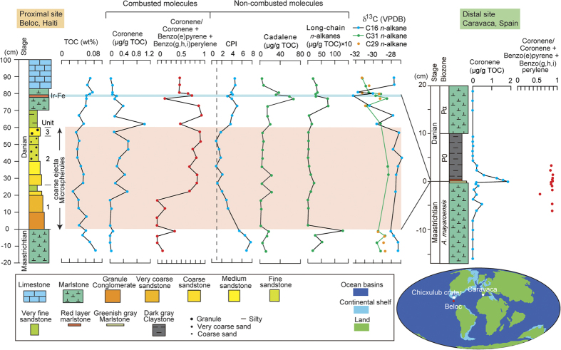
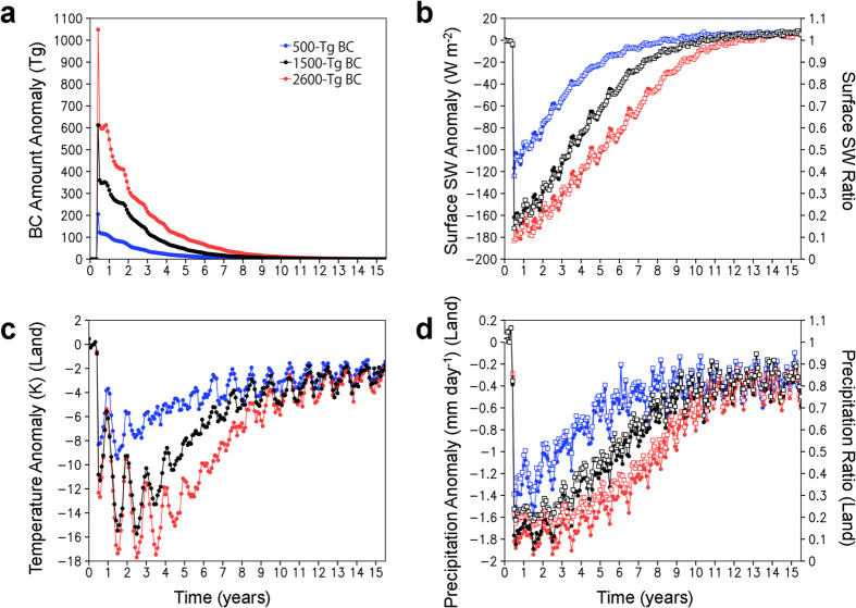
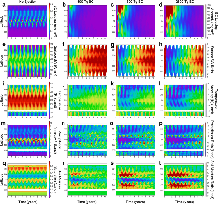
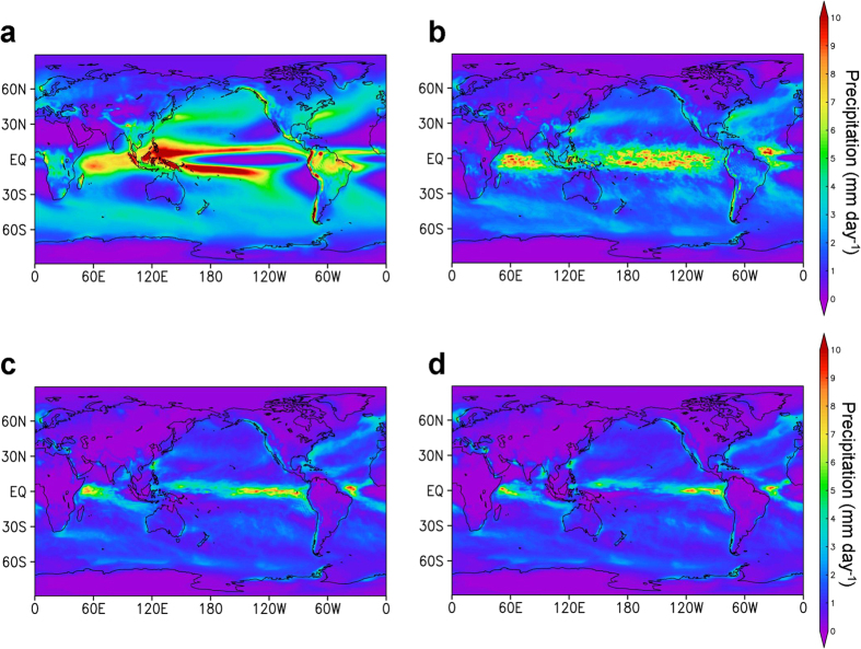
The mass extinction of life 66 million years ago at the Cretaceous/Paleogene boundary, marked by the extinctions of dinosaurs and shallow marine organisms, is important because it led to the macroevolution of mammals and appearance of humans. The current hypothesis for the extinction is that an asteroid impact in present-day Mexico formed condensed aerosols in the stratosphere, which caused the cessation of photosynthesis and global near-freezing conditions. Here, we show that the stratospheric aerosols did not induce darkness that resulted in milder cooling than previously thought. We propose a new hypothesis that latitude-dependent climate changes caused by massive stratospheric soot explain the known mortality and survival on land and in oceans at the Cretaceous/Paleogene boundary. The stratospheric soot was ejected from the oil-rich area by the asteroid impact and was spread globally. The soot aerosols caused sufficiently colder climates at mid–high latitudes and drought with milder cooling at low latitudes on land, in addition to causing limited cessation of photosynthesis in global oceans within a few months to two years after the impact, followed by surface-water cooling in global oceans in a few years. The rapid climate change induced terrestrial extinctions followed by marine extinctions over several years.
Overview
The claims and statistics of this paper haven’t been checked yet.
Run the check — free, no account needed. It reads the open-access text and checks the sources it cites.
Integrity signals
Registry
Cites
Statistics
Figures
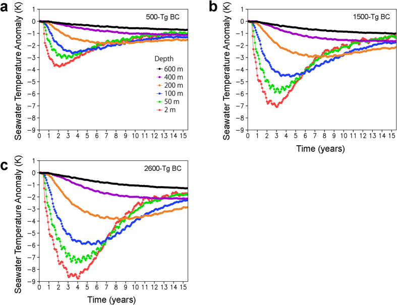
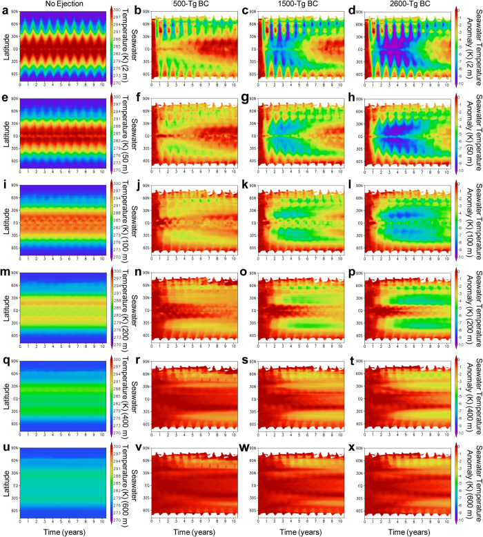
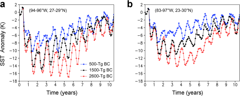
Verification
Claims the paper makes
The claims and statistics of this paper haven’t been checked yet.
Run the check — free, no account needed. It reads the open-access text and checks the sources it cites.
Claims other papers make about this one
Each is checked against this paper’s own text: does it say what the citing paper says it does?
In the citing paper
“This impactor struck carbonate and sulfate-rich sediments, leading to the ejection and global dispersal of large quantities of dust, ash, sulfur, and other aerosols into the atmosphere (4, 18–20).”
From Asteroid impact, not volcanism, caused the end-Cretaceous dinosaur extinction (2020) · cites this paper as [18]
In the citing paper
“An asteroid, ∼10 km in diameter, impacted at Chicxulub, in the present-day Gulf of Mexico, 66 Ma (4, 18, 19), leaving a crater ∼180 to 200 km in diameter (Fig. 1A).”
From Asteroid impact, not volcanism, caused the end-Cretaceous dinosaur extinction (2020) · cites this paper as [18]
Self-check
Percentages, sums and reported differences re-computed from the paper’s own numbers.
The self-check needs the paper’s full text.
Citations
Cites
No references could be resolved yet.
Research works printed but not linked: 67
- Alvarez, L. W., Alvarez, W., Asaro, F. & Michel, H. V. Extraterrestrial cause for the Cretaceous-Tertiary extinction. Science 208, 1095–1108 (1980). · DOI · Paper page
- Smit, J. & Hertogen, J. An extraterrestrial event at the Cretaceous-Tertiary boundary. Nature 285, 198–200 (1980). · DOI
- Hildebrand, A. R. et al. Chicxulub crater: A possible Cretaceous-Tertiary boundary impact crater on the Yucata’n Peninsula, Mexico. Geology 19, 867–871 (1991). · DOI · Paper page
- Schulte, P. et al. The Chicxulub Asteroid Impact and Mass Extinction at the Cretaceous-Paleogene Boundary. Science 327, 1214–1218 (2010). · DOI · Paper page
- Sheehan, P. M., Fastovsky, D. E., Barreto, C. & Hoffmann, R. G. Dinosaur abundance was not declining in a “3 m gap” at the top of the Hell Creek Formation, Montana and North Dakota. Geology 28, 523–526 (2000). · DOI
- Sheehan, P. M. & Fastovsky, D. E. Major extinction of land-dwelling vertebrates at the Cretaceous-Tertiary boundary, eastern Montana. Geology 20, 556–560 (1992). · DOI
- Landman, N. H., Garb, M. P., Rovelli, R., Ebel, D. S. & Edwards, L. E. Short–term survival of ammonites in New Jersey after the end–Cretaceous bolide impact. Acta Palaeontologica Polonica 57, 703–715 (2012). · DOI
- Landman, N. H., Goolaerts, S., Jagt, J. W. M., Jagt-Yazykova, E. A., Marcin Machalski, M. & Yacobucci, M. M. Ammonite extinction and nautilid survival at the end of the Cretaceous. Geology 42, 707–710 (2014). · DOI
- Zachos, J. C., Arthur, M. A. & Dean, W. E. Geochemical evidence for suppression of pelagic marine productivity at the Cretaceous/Tertiary boundary. Nature 337, 61–64 (1989). · DOI
- Kaiho, K. & Lamolda, M. A. Catastrophic extinction of planktonic forminifera at the Cretaceous-Tertiary boundary evidenced by stable isotopes and foraminiferal abundance at Caravaca, Spain. Geology 27, 355–358 (1999). · DOI · Paper page
- Norris, R. D., Huber, B. T. & Self-Trail, J. Synchroneity of the K–T oceanic mass extinction and meteorite impact: Blake Nose, western North Atlantic. Geology 27, 419–422 (1999).
- Kaiho, K. et al. Oceanic primary productivity and dissolved oxygen levels at the Cretaceous/Tertiary boundary: their decrease, subsequent warming and recovery. Paleoceanography 14, 511–524 (1999). · DOI
- D’Hondt, S. Consequences of the Cretaceous/Paleogene mass extinction for marine ecosystems. Annu. Rev. Ecol. Syst. 36, 295–317 (2005). · DOI
- Kaiho, K. Planktonic and benthic foraminiferal extinction events during the last 100 m.y. Palaeogeography Palaeoclimatology, Palaeoecology 111, 45–71 (1994). · DOI
- Robertson, D. S., McKenna, M. C., Toon, O. B., Hope, S. & Lillegraven, J. A. Survival in the first hours of the Cenozoic. Geol. Soc. Am. Bull. 116, 760–768, doi: 10.1120/B25402.1. (2004). · DOI
- Goldin, T. J. & Melosh, H. J. Self-shielding of thermal radiation by Chicxulub impact ejecta: Firestorm or fizzle? Geology 37, 1135–1138 (2009). · DOI
- Pope, K. O., Baines, K. H., Ocampo, A. C. & Ivanov, B. A. Energy, volatile production and climatic effects of the Chicxulub Cretaceous/Tertiary impact. J. Geophys. Res. 102(E9), 21645–21664 (1997). · DOI · Paper page
- Toon, O. B., Zahnle, K., Morrison, D., Turco, R. P. & Covey, C. Environmental perturbations caused by the impacts of asteroids and comets. Rev Geophys 35, 41 (1997). · DOI
- Pierazzo, E., Hahmann, A. N. & Sloan, L. C. Chicxulub and climate: radiative perturbations of impact-produced S-bearing gases. Astrobiology 3, 99–118 (2003). · DOI · Paper page
- Ohno, S. et al. Production of sulphate-rich vapour during the Chicxulub impact and implications for ocean acidification. Nature Geoscience 7, 279–282 (2014). · DOI
- Wolbach, W. S. Global fire at the Cretaceous–Tertiary boundary. Nature 334, 665–669 (1988). · DOI
- Bond, T. C. et al. Bounding the role of black carbon in the climate system: A scientific assessment. J. Geophys. Res. Atmos. 118, 5380–5552, doi: 10.1002/jgrd.50171 (2013). · DOI · Paper page
- Oshima, N. et al. Wet removal of black carbon in Asian outflow: Aerosol Radiative Forcing in East Asia (A-FORCE) aircraft campaign. J. Geophys. Res. 117, D03204, doi: 10.1029/2011JD016552 (2012). · DOI
- Maurasse, F. J.-M. R. & Sen, G. Impacts, Tsunamis and the Haitian Cretaceous-Tertiary Boundary Layer. Science 252, 1690–1693 (1991). · DOI
- Mizukami, T., Kaiho, K. & Oba, M. A spike of woody plant biomarkers in the deep-sea iridium layer at the Cretaceous/Paleogene boundary. Palaeogeogr., Palaeoclimatol., Palaeoecol. 412, 241–248 (2014). · DOI
- Richter, H. & Howard, J. B. Formation of polycyclic aromatic hydrocarbons and their growth to soot—a review of chemical reaction pathways. Progress in Energy and Combustion Science 26, 565–608 (2000). · DOI
- Wolbach, W. S. Cretaceous extinction: Evidence of wildfires and search for meteoritic material. Science 230, 160–170 (1985). · DOI
- Harvey, M. C., Brassell, S. C., Belcher, C. M. & Montanari, A. Combustion of fossil organic matter at the Cretaceous-Paleogene (K-P) boundary. Geology 36, 355–358 (2008). · DOI
- Belcher, C. M., Collinson, M. E., Sweet, A. R., Hildebrand, A. R. & Scott, A. C. “Fireball passes and nothing burns”—The role of thermal radiation in the K-T event: Evidence from the charcoal record of North America. Geology 31, 1061–1064 (2003). · DOI
- Sofiev, M., Vankevich, R., Ermakova, T. & Hakkarainen, J. Global mapping of maximum emission heights and resulting vertical profiles of wildfire emissions. Atmos. Chem. Phys. 13, 7039–7052, doi: 10.5194/acp-13-7039-2013 (2013). · DOI
- Wang, Y., Raj, A. & Chung, S. H. A PAH growth mechanism and synergistic effect on PAH formation in counter flow diffusion flames. Combustion and Flame 160, 1667–1676 (2013). · DOI
- Eglinton, G. & Hamilton, R. J. The distribution of n-alkanes. In Chemical Plant Taxonomy (ed. Swain, T. ), 187–217 (Academic Press, 1963). · DOI
- Simoneit, B. R. T. Organic matter of the troposphere-III. Characterization and sources of petroleum and pyrogenic residues in aerosols over the western United States. Atmos. Environ. 18, 51–67 (1984). · DOI
- Peters, K. E., Walters, C. C. & Moldowan, J. M. The Biomarker Guide. 473–1155 (Cambridge Univ. Press, 2005). · DOI
- Guzman-Vega, M. A. & Mello, M. R. Origin of oil in the Sureste Basin, Mexico: Am. Assoc. Petroleum Geologists Bull. 83, 1068–1095 (1999).
- Mizukami, T., Kaiho, K. & Oba, M. Significant changes in land vegetation and oceanic redox across the Cretaceous/Paleogene boundary. Palaeogeogr., Palaeoclimatol., Palaeoecol. 369, 41–47 (2013). · DOI
- Premovic, P. I. Soot in Cretaceous-Paleogene boundary clays worldwide: is it really derived from fossil fuel beds close to Chicxulub? Central European Journal of Geosciences 4, 383–387 (2012).
- Wang, H. Formation of nascent soot and other condensed-phase materials in flames. Proceedings of the Combustion Institute 33, 41–67 (2011). · DOI
- Robertson, D. S., Lewis, W. M., Sheehan, P. M. & Toon, O. B. K-Pg extinction: Reevaluation of the heat-fire hypothesis. J. Geophys. Res: Biogeosci. 118, 329–336, doi: 10.1002/jgrg.20018.41 (2013). · DOI
- Upchurch, G. R., Jr, Otto-Bliesner, B. L. & Scotese, C. Vegetation±atmosphere interactions and their role in global warming during the latest Cretaceous. Phil. Trans. R. Soc. Lond. B 353, 97–112 (1998). · DOI
- Floegel, S. & Wagner, T. Insolation-control on the Late Cretaceous hydrological cycle and tropical African climate—global climate modelling linked to marine climate records. Palaeogeogr., Palaeoclimatol., Palaeoecol. 235, 288–304 (2006). · DOI
- Bush, A. B. G. & Philander, S. G. H. The late Cretaceous: Simulation with a coupled atmosphere-ocean general circulation model. Paleoceanography 12, 495–516 (1997). · DOI
- Grajales-Nishimura, J. M. et al. Chicxulub impact: The origin of reservoir and seal facies in the southeastern Mexico oil fields. Geology 28, 307–310 (2000). · DOI
- Vellekoop, J. et al. Rapid short-term cooling following the Chicxulub impact at the Cretaceous–Paleogene boundary. Proc. Natl. Acad. Sci. USA 111, 7537–7541 (2014). · DOI · Paper page
- Sitch, S. et al. Evaluation of ecosystem dynamics, plant geography and terrestrial carbon cycling in the LPJ dynamic global vegetation model. Global Change Biology 9, 161–185 (2003). · DOI
- Mannion, P. D. et al. Temperate palaeodiversity peak in Mesozoic dinosaurs and evidence for Late Cretaceous geographical partitioning. Global Ecol. Biogeogr. 21, 898–908 (2012). · DOI
- Watanabe, A., Erickson, G. M. & Druckenmiller, P. S. An ornithomimosaurian from the Upper Cretaceous Prince Creek Formation of Alaska. J. Vertebrate Paleontol. 33, 1169–1175 (2013). · DOI
- Barazaitis, P. & Watanabe, M. E. Crocodilian behaviour: a window to dinosaur behaviour? Historical Biology 23, 73–90 (2011). · DOI
- Lance, V. A. Alligator physiology and life history: the importance of temperature. Exp Gerontol. 38, 801–805 (2003) · DOI
- Farlow, J., Dodson, P. & Chinsamy, A. Dinosaur Biology. Annual Review of Ecology and Systematics 26, 445–471 (1995). · DOI
- Sessa, J. A. et al. Ammonite habitat revealed via isotopic composition and comparisons with co-occurring benthic and planktonic organisms. PNAS 112, 15562–15567 (2015). · DOI
- Henderson, R. A. & Price, G. D. Paleoenvironment and paleoecology inferred from oxygen and carbon isotopes of subtropical mollusks from the late cretaceous (Cenomanian) of Bathurst Island, Australia. Palaios 27, 617–626 (2012). · DOI
- Dennis, K. J., Cochran, J. K., Landman, N. H. & Schrag, D. P. The climate of the Late Cretaceous: New insights from the application of the carbonate clumped isotope thermometer to Western Interior Seaway macrofossil. Earth and Planetary Science Letters 362, 51–65 (2013). · DOI
- Kruta, I., Landman, N. H. & Cochran, J. K. A new approach for the determination of ammonite and nautilid habtats. PLoS ONE 9(1), e87479. doi: 10.1371/journal.pone.0087479 (2014). · DOI
- Lukeneder, A., Harzhauser, M., Müllegger, S. & Piller, W. E. Ontogeny and habitat change in Mesozoic cephalopods revealed by stable isotopes (δ18O, δ13C). Earth and Planetary Science Letters 296, 103–114 (2010). · DOI
- Stevens, K., Mutterlose, J. & Wiedenroth, K. Stable isotope data (δ18O, δ13C) of the ammonite genus Simbirskites — implications for habitat reconstructions of extinct cephalopods. Palaeogeography, Palaeoclimatology, Palaeoecology 417, 164–175 (2015). · DOI
- Kaiho, K. Planktonic and benthic foraminiferal extinction events during the last 100 m.y. Palaeogeogr. Palaeoclimatol., Palaeoecol. 111, 45–71 (1994). · DOI
- Oba, T., Kai, M. & Tanabe, K. Early life history and habitat of Nautilus pompilius inferred from oxygen isotope examinations. Marine Biology 113, 211–217 (1992). · DOI
- Liu, N., Peng, C. L., Lin, Z. F., Lin, G. Z. & Pan, X. P. Regulation of light energy utilization and distribution of photosynthesis in five subtropical woody plants. J. Integr. Plant Biol. 49, 351–361 (2007). · DOI
- Paulson, C. A. & Simpson, J. J. Irradiance measurements in the upper ocean, J. Phys. Oceanogr. 7, 952–956 (1977). · DOI
- Lamolda, M. A., Melinte, M. C. & Kaiho, K. Nannofloral extinction and survivorship across the K/T boundary at Caravaca, southeastern Spain. Palaeogeogr, Palaeoclimatol, Palaeoecol 224, 27–52 (2005). · DOI
- Mayor, A. G. et al. Feedbacks between vegetation pattern and resource loss dramatically decrease ecosystem resilience and restoration potential in a simple dryland model. Landscape Ecol. 28, 931–942 (2013). · DOI
- Fuls, E. R. Ecosystem modification created by patch-overgrazing in semi-arid grassland. J. Arid Environments 23, 59–69 (1992). · DOI
- D’Odorico, P. et al. Global desertification: Drivers and feedbacks. Advances in Water Resources 51, 326–344 (2013). · DOI
- Mazzotti, F. J. et al. Alligators and crocodiles as indicators for restoration of Everglades ecosystems. Ecological Indicators 9s, s137–s149 (2009). · DOI
- Yukimoto, S. et al. A new global climate model of the Meteorological Research Institute: MRI-CGCM3 -Model description and basic performance-. J. Meteor. Soc. Japan 90A, 23–64, doi: 10.2151/jmsj.2012-A02 (2012). · DOI
- Courtillot, V., Jaupart, C., Manighetti, P. & Besse, J. On causal links between flood basalts and continental breakup. Earth and Planetary Science Letters. 166, 177–195 (1999). · DOI
Cited by
Asteroid impact, not volcanism, caused the end-Cretaceous dinosaur extinction
Chiarenza, A. A., Farnsworth, A., Mannion, P. D., Lunt, D. J., Valdes, P. J., Morgan, J. V., & Allison, P. A. (2020) · Proceedings of the National Academy of Sciences · doi:10.1073/pnas.2006087117 · Cited by 228
Metadata
- Authors
- Kaiho, K., Oshima, N., Adachi, K., Adachi, Y., Mizukami, T., Fujibayashi, M., & Saito, R.
- Venue
- Scientific Reports
- Published
- 2016-07-14
- Volume
- 6
- Issue
- 1
- ISSN
- 2045-2322
- PMC
- PMC4944614
- Cited by
- 105
- References
- 0
- Language
- en
About these checks
Registry, retraction, Cites and statistics results are computed, not judged, with one exception: a printed reference that no index lists is read once by a model before it counts as a citation error. Claims are extracted by a model and kept only when their quote appears verbatim in the text; each cited source is then checked, with a model’s help, for whether it says what the claim relies on. Those verdicts can be wrong — read the claim’s quote and the cited source before relying on one.
Statistics and arithmetic are recomputed, not judged.
Confidence bands are shown only for fields calibrated on our annotated test set. None is calibrated yet, so no band is shown.
What counts as a claim ›How we measure confidence ›How we check this ›
Are you an author, or do you see a problem with this page? Request a review
