Student or educator? Sign up with your school email and get 6 months of Pro free.
Cited by 2,442

The DOI matches its Crossref record; 305 of the 305 references it cites were found in a registry or an index.

Planck 2018 results: X. Constraints on inflation

Planck Collaboration, Akrami, Y., Arroja, F., Ashdown, M., Aumont, J., Baccigalupi, C., Ballardini, M., Banday, A. J., Barreiro, R. B., Bartolo, N., Basak, S., Benabed, K., Bernard, J.-P., Bersanelli, M., Bielewicz, P., Bock, J. J., Bond, J. R., Borrill, J., Bouchet, F. R., Boulanger, F., Bucher, M., Burigana, C., Butler, R. C., Calabrese, E., Cardoso, J.-F., Carron, J., Challinor, A., Chiang, H. C., Colombo, L. P. L., Combet, C., Contreras, D., Crill, B. P., Cuttaia, F., de Bernardis, P., de Zotti, G., Delabrouille, J., Delouis, J.-M., Di Valentino, E., Diego, J. M., Donzelli, S., Doré, O., Douspis, M., Ducout, A., Dupac, X., Dusini, S., Efstathiou, G., Elsner, F., Enßlin, T. A., Eriksen, H. K., Fantaye, Y., Fergusson, J., Fernandez-Cobos, R., Finelli, F., Forastieri, F., Frailis, M., Franceschi, E., Frolov, A., Galeotta, S., Galli, S., Ganga, K., Gauthier, C., Génova-Santos, R. T., Gerbino, M., Ghosh, T., González-Nuevo, J., Górski, K. M., Gratton, S., Gruppuso, A., Gudmundsson, J. E., Hamann, J., Handley, W., Hansen, F. K., Herranz, D., Hivon, E., Hooper, D. C., Huang, Z., Jaffe, A. H., Jones, W. C., Keihänen, E., Keskitalo, R., Kiiveri, K., Kim, J., Kisner, T. S., Krachmalnicoff, N., Kunz, M., Kurki-Suonio, H., Lagache, G., Lamarre, J.-M., Lasenby, A., Lattanzi, M., Lawrence, C. R., Le Jeune, M., Lesgourgues, J., Levrier, F., Lewis, A., Liguori, M., Lilje, P. B., Lindholm, V., López-Caniego, M., Lubin, P. M., Ma, Y.-Z., Macías-Pérez, J. F., Maggio, G., Maino, D., Mandolesi, N., Mangilli, A., Marcos-Caballero, A., Maris, M., Martin, P. G., Martínez-González, E., Matarrese, S., Mauri, N., McEwen, J. D., Meerburg, P. D., Meinhold, P. R., Melchiorri, A., Mennella, A., Migliaccio, M., Mitra, S., Miville-Deschênes, M.-A., Molinari, D., Moneti, A., Montier, L., Morgante, G., Moss, A., Münchmeyer, M., Natoli, P., Nørgaard-Nielsen, H. U., Pagano, L., Paoletti, D., Partridge, B., Patanchon, G., Peiris, H. V., Perrotta, F., Pettorino, V., Piacentini, F., Polastri, L., Polenta, G., Puget, J.-L., Rachen, J. P., Reinecke, M., Remazeilles, M., Renzi, A., Rocha, G., Rosset, C., Roudier, G., Rubiño-Martín, J. A., Ruiz-Granados, B., Salvati, L., Sandri, M., Savelainen, M., Scott, D., Shellard, E. P. S., Shiraishi, M., Sirignano, C., Sirri, G., Spencer, L. D., Sunyaev, R., Suur-Uski, A.-S., Tauber, J. A., Tavagnacco, D., Tenti, M., Toffolatti, L., Tomasi, M., Trombetti, T., Valiviita, J., Van Tent, B., Vielva, P., Villa, F., Vittorio, N., Wandelt, B. D., Wehus, I. K., White, S. D. M., Zacchei, A., Zibin, J. P., Zonca, A.·2020·Astronomy & Astrophysics

Abstract

We report on the implications for cosmic inflation of the 2018 release of the Planck cosmic microwave background (CMB) anisotropy measurements. The results are fully consistent with those reported using the data from the two previous Planck cosmological releases, but have smaller uncertainties thanks to improvements in the characterization of polarization at low and high multipoles. Planck temperature, polarization, and lensing data determine the spectral index of scalar perturbations to be n s = 0.9649 ± 0.0042 at 68% CL. We find no evidence for a scale dependence of n s , either as a running or as a running of the running. The Universe is found to be consistent with spatial flatness with a precision of 0.4% at 95% CL by combining Planck with a compilation of baryon acoustic oscillation data. The Planck 95% CL upper limit on the tensor-to-scalar ratio, r 0.002 < 0.10, is further tightened by combining with the BICEP2/Keck Array BK15 data to obtain r 0.002 < 0.056. In the framework of standard single-field inflationary models with Einstein gravity, these results imply that: (a) the predictions of slow-roll models with a concave potential, V ″( ϕ ) < 0, are increasingly favoured by the data; and (b) based on two different methods for reconstructing the inflaton potential, we find no evidence for dynamics beyond slow roll. Three different methods for the non-parametric reconstruction of the primordial power spectrum consistently confirm a pure power law in the range of comoving scales 0.005 Mpc −1 ≲ k ≲ 0.2 Mpc −1 . A complementary analysis also finds no evidence for theoretically motivated parameterized features in the Planck power spectra. For the case of oscillatory features that are logarithmic or linear in k , this result is further strengthened by a new combined analysis including the Planck bispectrum data. The new Planck polarization data provide a stringent test of the adiabaticity of the initial conditions for the cosmological fluctuations. In correlated, mixed adiabatic and isocurvature models, the non-adiabatic contribution to the observed CMB temperature variance is constrained to 1.3%, 1.7%, and 1.7% at 95% CL for cold dark matter, neutrino density, and neutrino velocity, respectively. Planck power spectra plus lensing set constraints on the amplitude of compensated cold dark matter-baryon isocurvature perturbations that are consistent with current complementary measurements. The polarization data also provide improved constraints on inflationary models that predict a small statistically anisotropic quadupolar modulation of the primordial fluctuations. However, the polarization data do not support physical models for a scale-dependent dipolar modulation. All these findings support the key predictions of the standard single-field inflationary models, which will be further tested by future cosmological observations.

Overview

The claims and statistics of this paper haven’t been checked yet.

Run the check — free, no account needed. It reads the open-access text and checks the sources it cites.

A few free checks a day · papers already verified open instantly · results are public

Integrity signals

Registry

Crossref · 10.1051/0004-6361/201833887

Cites

305 of 305 references verified0 citation errors · 0 not checkable

Statistics

Figures
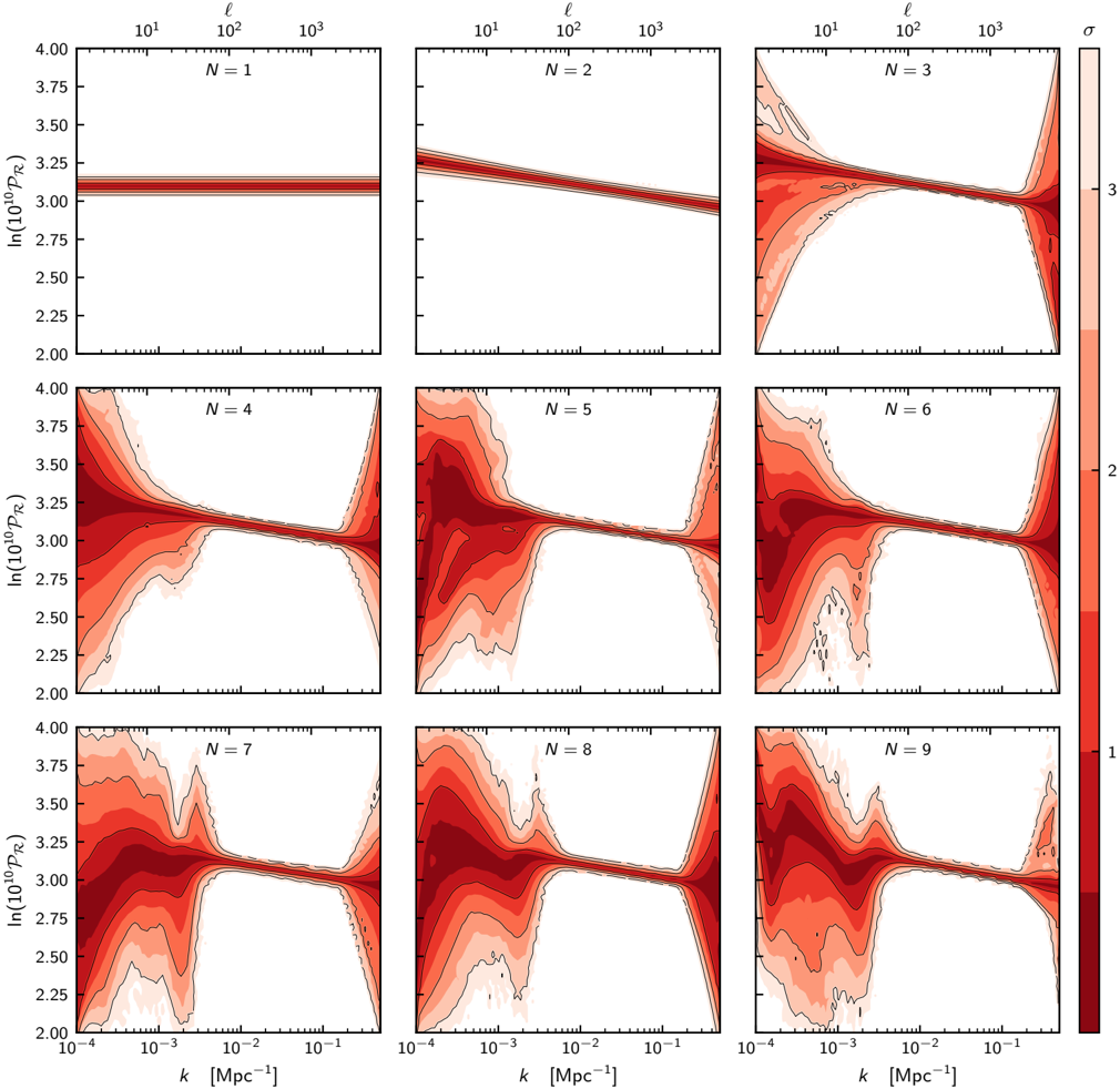
Image 1
CC-BY · From the PDF
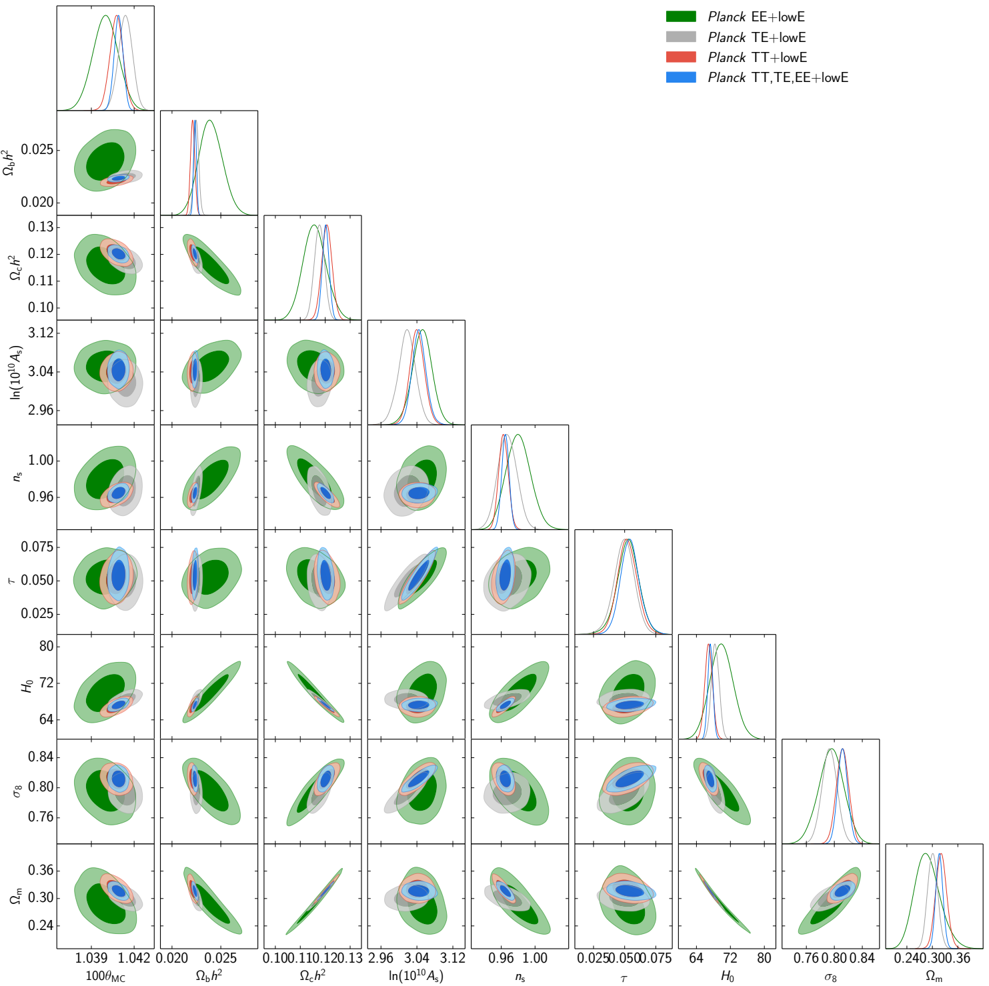
Fig. 2 Marginalized joint 68% and 95% CL regions for the cosmological parameters in CDM with Planck TT, EE, TE, and joint TT,TE,EE, all in combination with the EE likelihood at low multipoles.
Fig. 2 Marginalized joint 68% and 95% CL regions for the cosmological parameters in CDM with Planck TT, EE, TE, and joint TT,TE,EE, all in combination with the EE likelihood at low multipoles.CC-BY · From the PDF
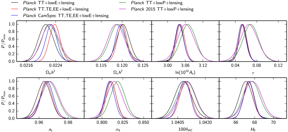
Fig. 3 Comparison of the marginalized probability density of the primary parameters and ( 8 ; H 0 ) for the baseline cosmological model from Planck TT + lowE + lensing (black curves), TT,TE,EE + lowE + lensing (red curves), and the alternative likelihood Camspec . For comparison we also display the Planck 2018 TT + lowP + lensing (blue curves) and the corresponding Planck 2015 TT + lowP + lensing (green curves) results.
Fig. 3 Comparison of the marginalized probability density of the primary parameters and ( 8 ; H 0 ) for the baseline cosmological model from Planck TT + lowE + lensing (black curves), TT,TE,EE + lowE + lensing (red curves), and the alternative likelihood Camspec . For comparison we also display the Planck 2018 TT + lowP + lensing (blue curves) and the corresponding Planck 2015 TT + lowP + lensing (green curves) results.CC-BY · From the PDF
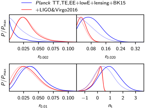
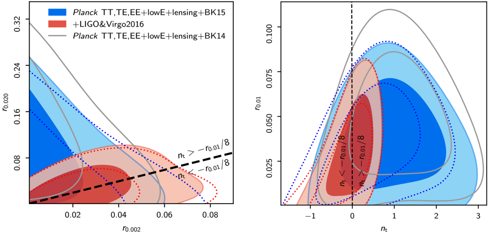
Fig. 4 Posterior probability density of the tensor-to-scalar ratio at two di erent scales in the CDM + r 0 : 002 + r 0 : 02 model, i.e., when the inflationary consistency relation is relaxed ( top panels ). The solid contours show the results when r 0 : 002 and r 0 : 02 are used as sampling parameters with uniform priors, which leads to non-uniform priors for the derived parameters r 0 : 01 and n t ( bottom panels ). The dotted contours indicate the results after weighting the posterior by the Jacobian J = r 0 : 01 = [ r 0 : 002 r 0 : 02 ln(0 : 02 = 0 : 002)] of the transformation ( r 0 : 002 ; r 0 : 02 ) ! ( r 0 : 01 ; n t ), giving the result we would have obtained had we assigned uniform priors on r 0 : 01 and n t .
Fig. 4 Posterior probability density of the tensor-to-scalar ratio at two di erent scales in the CDM + r 0 : 002 + r 0 : 02 model, i.e., when the inflationary consistency relation is relaxed ( top panels ). The solid contours show the results when r 0 : 002 and r 0 : 02 are used as sampling parameters with uniform priors, which leads to non-uniform priors for the derived parameters r 0 : 01 and n t ( bottom panels ). The dotted contours indicate the results after weighting the posterior by the Jacobian J = r 0 : 01 = [ r 0 : 002 r 0 : 02 ln(0 : 02 = 0 : 002)] of the transformation ( r 0 : 002 ; r 0 : 02 ) ! ( r 0 : 01 ; n t ), giving the result we would have obtained had we assigned uniform priors on r 0 : 01 and n t .CC-BY · From the PDF
Image 5
CC-BY · From the PDF
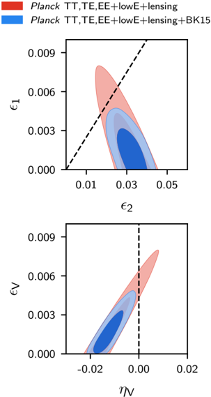
Fig. 6 Marginalized joint two-dimensional 68% and 95% CL regions for ( 1 ; 2 ) ( top panel ) and ( V ; V ) ( bottom panel ) for Planck TT,TE,EE + lowE + lensing (red contours), compared with Planck TT,TE,EE + lowE + lensing + BK15 (blue contours). The dashed lines divide between convex and concave potentials.
Fig. 6 Marginalized joint two-dimensional 68% and 95% CL regions for ( 1 ; 2 ) ( top panel ) and ( V ; V ) ( bottom panel ) for Planck TT,TE,EE + lowE + lensing (red contours), compared with Planck TT,TE,EE + lowE + lensing + BK15 (blue contours). The dashed lines divide between convex and concave potentials.CC-BY · From the PDF
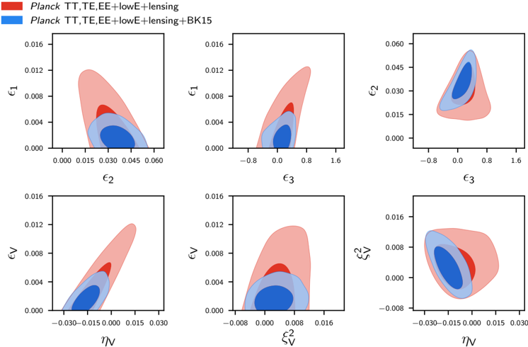
Fig. 7 Marginalized joint two-dimensional 68% and 95% CL regions for combinations of ( 1 ; 2 ; 3 ) ( upper panels ) and ( V ; V ; 2 V ) ( lower panels ) for Planck TT,TE,EE + lowE + lensing (red contours), compared with Planck TT,TE,EE + lowE + lensing + BK15 (blue contours).
Fig. 7 Marginalized joint two-dimensional 68% and 95% CL regions for combinations of ( 1 ; 2 ; 3 ) ( upper panels ) and ( V ; V ; 2 V ) ( lower panels ) for Planck TT,TE,EE + lowE + lensing (red contours), compared with Planck TT,TE,EE + lowE + lensing + BK15 (blue contours).CC-BY · From the PDF
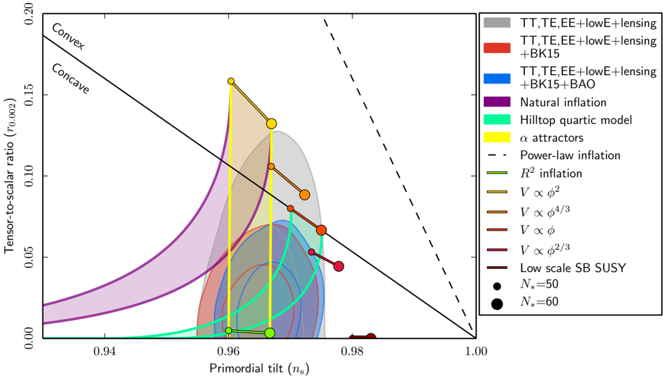
Fig. 8 Marginalized joint 68% and 95% CL regions for n s and r at k = 0 : 002 Mpc 1 from Planck alone and in combination with BK15 or BK15 + BAO data, compared to the theoretical predictions of selected inflationary models. Note that the marginalized joint 68% and 95% CL regions assume d n s = d ln k = 0.
Fig. 8 Marginalized joint 68% and 95% CL regions for n s and r at k = 0 : 002 Mpc 1 from Planck alone and in combination with BK15 or BK15 + BAO data, compared to the theoretical predictions of selected inflationary models. Note that the marginalized joint 68% and 95% CL regions assume d n s = d ln k = 0.CC-BY · From the PDF
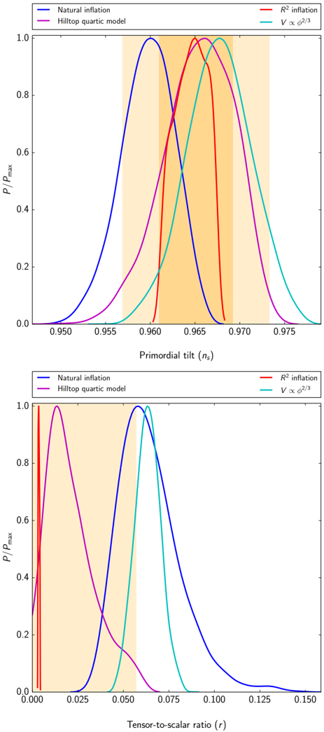
Fig. 9 Marginalized probability densities of the scalar tilt n s ( top panel ) and r ( bottom panel ) at k = 0 : 002 Mpc 1 for natural, R 2 , hilltop quartic, and V ( ) / 2 = 3 inflation, obtained by marginalizing over the uncertainties in the entropy generation stage, compared to the corresponding 68% and 95% CL limits obtained from a CDM-plus-tensor fit.
Fig. 9 Marginalized probability densities of the scalar tilt n s ( top panel ) and r ( bottom panel ) at k = 0 : 002 Mpc 1 for natural, R 2 , hilltop quartic, and V ( ) / 2 = 3 inflation, obtained by marginalizing over the uncertainties in the entropy generation stage, compared to the corresponding 68% and 95% CL limits obtained from a CDM-plus-tensor fit.CC-BY · From the PDF
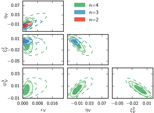
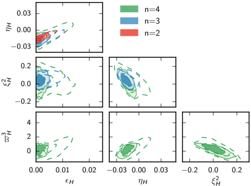
Fig. 10 Taylor expansion of V ( ) at order n = 2, 3, and 4 in the observable region, making no assumption about the end of inflation. The parameters are combinations of Taylor coe cients with flat priors. Dashed contours are Planck TT,TE,EE + lowE, while solid contours are Planck TT,TE,EE + lowE + lensing + BK15. The scales are the same as in PCI15.
Fig. 10 Taylor expansion of V ( ) at order n = 2, 3, and 4 in the observable region, making no assumption about the end of inflation. The parameters are combinations of Taylor coe cients with flat priors. Dashed contours are Planck TT,TE,EE + lowE, while solid contours are Planck TT,TE,EE + lowE + lensing + BK15. The scales are the same as in PCI15.CC-BY · From the PDF
Image 11
CC-BY · From the PDF
Image 12
CC-BY · From the PDF
Notes. We also show the corresponding bounds on some related parameters (here n s , d n s = d ln k , and r 0 : 002 are derived from the numerically computed primordial spectra). All error bars are at the 68% CL and all upper bounds at the 95% CL. The e ective 2 value of model n is given relative to model n 1.
Notes. We also show the corresponding bounds on some related parameters (here n s , d n s = d ln k , and r 0 : 002 are derived from the numerically computed primordial spectra). All error bars are at the 68% CL and all upper bounds at the 95% CL. The e ective 2 value of model n is given relative to model n 1.CC-BY · From the PDF
Image 14
CC-BY · From the PDF
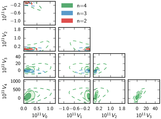
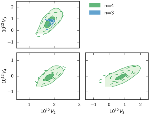
Fig. 15 Taylor expansion of the full V ( ) at order n = 3 and 4, trusted until the end of inflation, in natural units (where p 8 M Pl = 1). The parameters are the Taylor coe cients with flat priors. Dashed contours are Planck TT,TE,EE + lowE, while solid contours are Planck TT,TE,EE + lowE + lensing + BK15.
Fig. 15 Taylor expansion of the full V ( ) at order n = 3 and 4, trusted until the end of inflation, in natural units (where p 8 M Pl = 1). The parameters are the Taylor coe cients with flat priors. Dashed contours are Planck TT,TE,EE + lowE, while solid contours are Planck TT,TE,EE + lowE + lensing + BK15.CC-BY · From the PDF
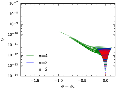
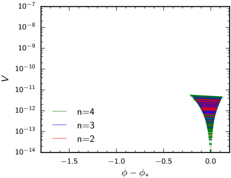
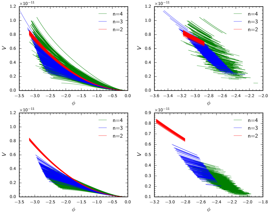
Fig. 16 Representative sample of the inflation potentials allowed at the 95% CL, when the potential is Taylor-expanded at order n = 2, 3, and 4 and trusted until the end of inflation, and under the assumption of N = 55 e -folds of inflation between Hubble-radius crossing for the pivot scale and the end of inflation. In natural units (where p 8 M Pl = 1). Left panels : full potential from the beginning of the observable window till the end of inflation. Right : zoom on the observable window directly constrained by inflation. Top : Planck TT,TE,EE + lowE. Bottom : Planck TT,TE,EE + lowE + lensing + BK15. Note that there is another branch of solutions that is symmetric under ! .
Fig. 16 Representative sample of the inflation potentials allowed at the 95% CL, when the potential is Taylor-expanded at order n = 2, 3, and 4 and trusted until the end of inflation, and under the assumption of N = 55 e -folds of inflation between Hubble-radius crossing for the pivot scale and the end of inflation. In natural units (where p 8 M Pl = 1). Left panels : full potential from the beginning of the observable window till the end of inflation. Right : zoom on the observable window directly constrained by inflation. Top : Planck TT,TE,EE + lowE. Bottom : Planck TT,TE,EE + lowE + lensing + BK15. Note that there is another branch of solutions that is symmetric under ! .CC-BY · From the PDF
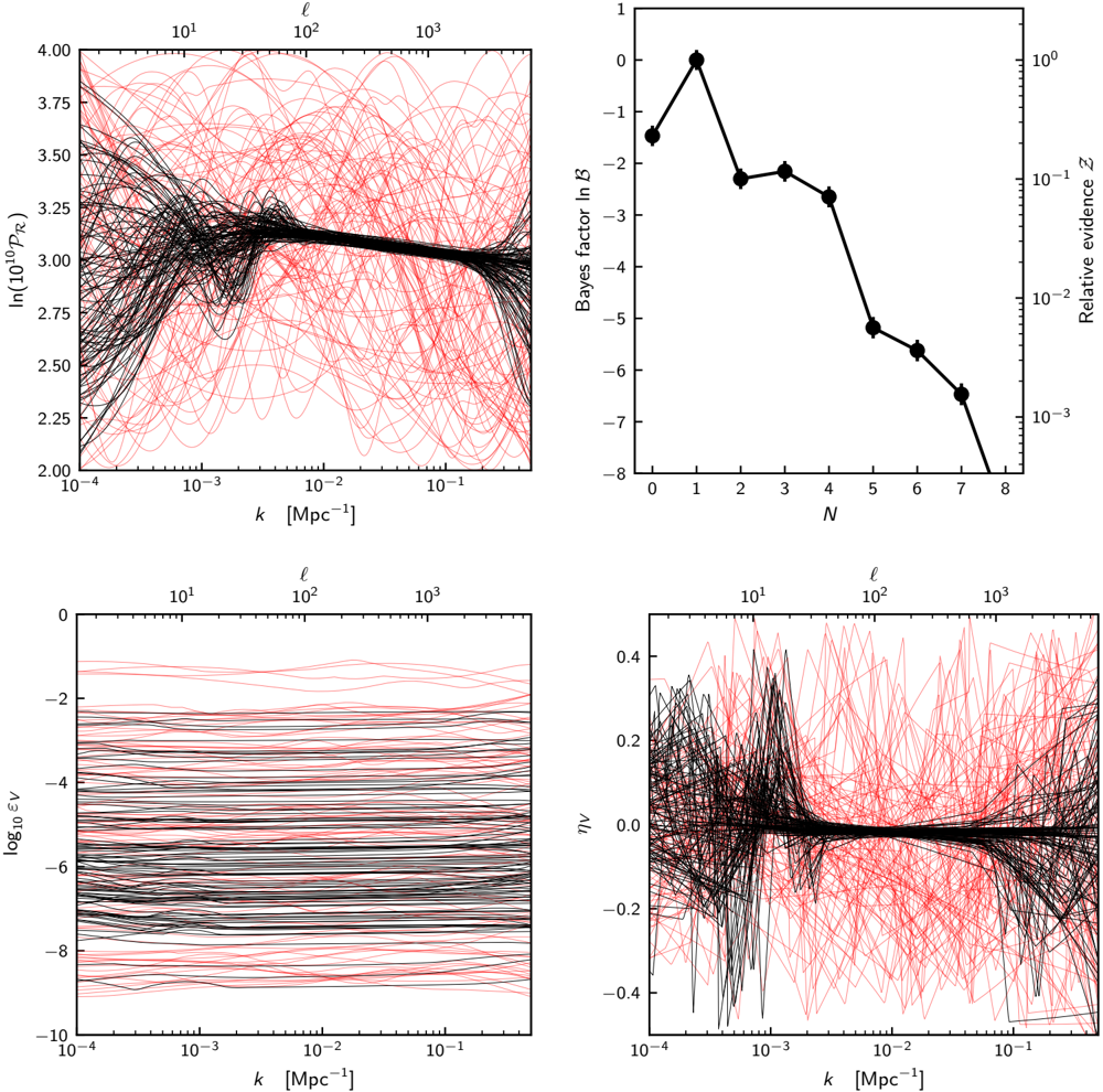
Fig. 17 Free-form potential reconstructions using Planck TT + TE + EE + lowE + lensing (Sect. 5.4). Top-right panel : Bayes factors for the free-form potential reconstruction. The preferred reconstruction has N = 1, corresponding to a constant non-zero d 2 ln V 1 = d 2 . The remaining panels show reconstructions for the N = 8 knot case, focusing on the scalar primordial power spectrum, and the inflationary slow-roll parameters " V and V . Red lines indicate sample trajectories from the prior, whilst black lines are from the posterior. Technically the slow-roll parameters are defined as functions of , but we instead substitute this for the Hubble-radius-exit value to make for clearer comparison between posterior samples. In all plots, the approximate link between ' and k is via the Limber approximation, ' ' k = D A, where D A = r = is the comoving angular distance to recombination, which is at comoving distance r .
Fig. 17 Free-form potential reconstructions using Planck TT + TE + EE + lowE + lensing (Sect. 5.4). Top-right panel : Bayes factors for the free-form potential reconstruction. The preferred reconstruction has N = 1, corresponding to a constant non-zero d 2 ln V 1 = d 2 . The remaining panels show reconstructions for the N = 8 knot case, focusing on the scalar primordial power spectrum, and the inflationary slow-roll parameters " V and V . Red lines indicate sample trajectories from the prior, whilst black lines are from the posterior. Technically the slow-roll parameters are defined as functions of , but we instead substitute this for the Hubble-radius-exit value to make for clearer comparison between posterior samples. In all plots, the approximate link between ' and k is via the Limber approximation, ' ' k = D A, where D A = r = is the comoving angular distance to recombination, which is at comoving distance r .CC-BY · From the PDF
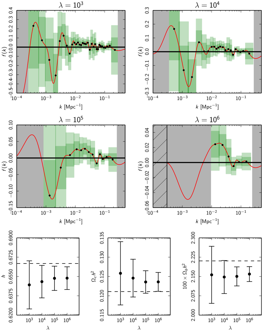
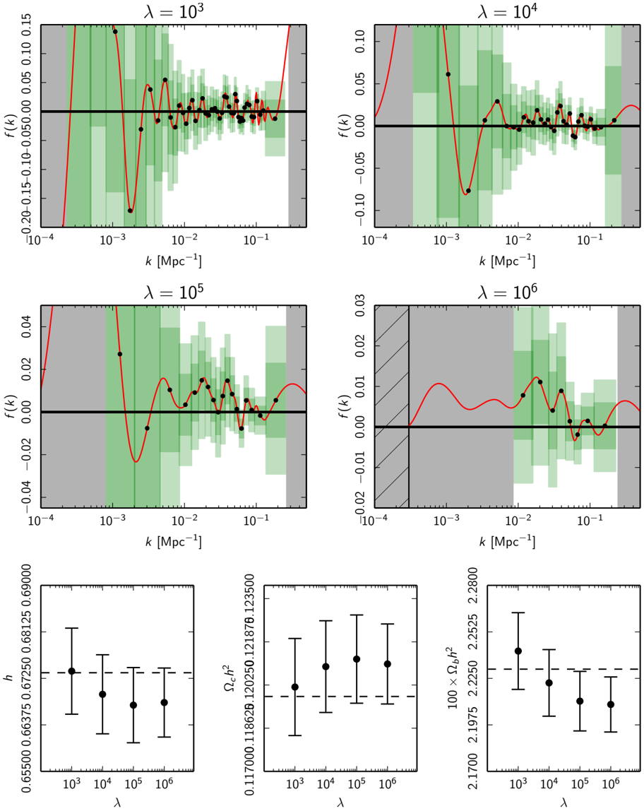
Fig. 18 Planck TT + lowE penalized likelihood primordial power spectrum reconstruction. Top four panels : deviation f ( k ) for four di erent roughness penalties. The red curves indicate the best-fit deviation, while the vertical extents of the dark and light green error bars indicate the 1 and 2 errors, respectively. The width of the error bars indicates the minimum reconstructible width (the minimum width for a Gaussian feature such that the mean square deviation of the reconstruction is less than 10%). The grey regions display where the minimum reconstructible width is undefined, meaning that the reconstruction in these regions is untrustworthy. The hatched region in the = 10 6 plot indicates where the fixing penalty has been applied. Lower three panels : 1 error bars for the three non-primordial-specctrum cosmological parameters included in the reconstruction. The respective best-fit fiducial model values are indicated by the dashed lines.
Fig. 18 Planck TT + lowE penalized likelihood primordial power spectrum reconstruction. Top four panels : deviation f ( k ) for four di erent roughness penalties. The red curves indicate the best-fit deviation, while the vertical extents of the dark and light green error bars indicate the 1 and 2 errors, respectively. The width of the error bars indicates the minimum reconstructible width (the minimum width for a Gaussian feature such that the mean square deviation of the reconstruction is less than 10%). The grey regions display where the minimum reconstructible width is undefined, meaning that the reconstruction in these regions is untrustworthy. The hatched region in the = 10 6 plot indicates where the fixing penalty has been applied. Lower three panels : 1 error bars for the three non-primordial-specctrum cosmological parameters included in the reconstruction. The respective best-fit fiducial model values are indicated by the dashed lines.CC-BY · From the PDF
Fig. 19 Penalized likelihood reconstruction, as Fig. 18 but for Planck TT,TE,EE + lowE.
Fig. 19 Penalized likelihood reconstruction, as Fig. 18 but for Planck TT,TE,EE + lowE.CC-BY · From the PDF
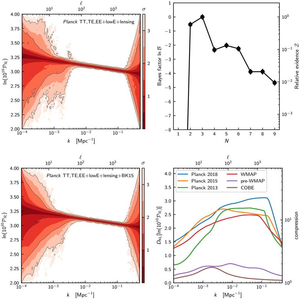
Fig. 20 Free-form Bayesian reconstruction of the primordial power spectrum (Sect. 6.2.1) using Planck TT,TE,EE + lowE + lensing. Top-right : evidence values for each N -knot reconstruction. The evidence is maximal for the N = 2 and N = 3 knot cases, and semi-competitive for the remaining higher knots. Marginalizing over the number of knots produces a predictive posterior plot, shown in the top-left panel . Here we see generic features, with the limit of resolution of Planck at ' ' 2400 and cosmic variance at low ' . Bottom-left : same as top-left, but using the additional BK15 data and allowing r to vary. Bottom-right : Kullback-Leibler divergence conditional on k , marginalized over the number of knots, showing the increase in compression of the primordial power spectrum over several past CMB missions. The di erence in constraining power between Planck 2013 and 2015 is driven entirely by the shift in the constraint.
Fig. 20 Free-form Bayesian reconstruction of the primordial power spectrum (Sect. 6.2.1) using Planck TT,TE,EE + lowE + lensing. Top-right : evidence values for each N -knot reconstruction. The evidence is maximal for the N = 2 and N = 3 knot cases, and semi-competitive for the remaining higher knots. Marginalizing over the number of knots produces a predictive posterior plot, shown in the top-left panel . Here we see generic features, with the limit of resolution of Planck at ' ' 2400 and cosmic variance at low ' . Bottom-left : same as top-left, but using the additional BK15 data and allowing r to vary. Bottom-right : Kullback-Leibler divergence conditional on k , marginalized over the number of knots, showing the increase in compression of the primordial power spectrum over several past CMB missions. The di erence in constraining power between Planck 2013 and 2015 is driven entirely by the shift in the constraint.CC-BY · From the PDF
Fig. 21 Free-form Bayesian reconstruction of the primordial power spectrum for varying numbers of knots (Sect. 6.2.1) using TT,TE,EE + lowE + lensing. The amplitude and tilt are consistent with the rest of the results with the same combination of likelihoods. As more knots are added, the ' ' 30 feature in the C ' temperature spectrum is visible as a dip to lower power.
Fig. 21 Free-form Bayesian reconstruction of the primordial power spectrum for varying numbers of knots (Sect. 6.2.1) using TT,TE,EE + lowE + lensing. The amplitude and tilt are consistent with the rest of the results with the same combination of likelihoods. As more knots are added, the ' ' 30 feature in the C ' temperature spectrum is visible as a dip to lower power.CC-BY · From the PDF
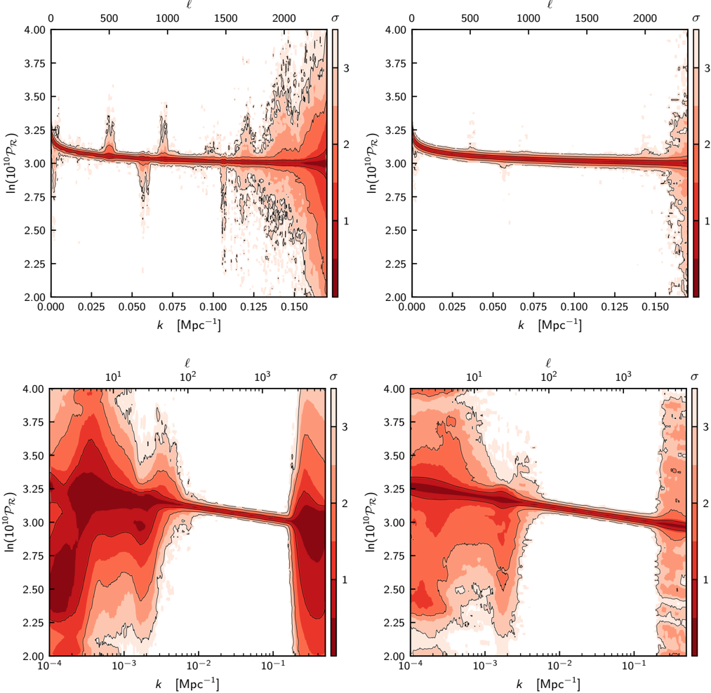
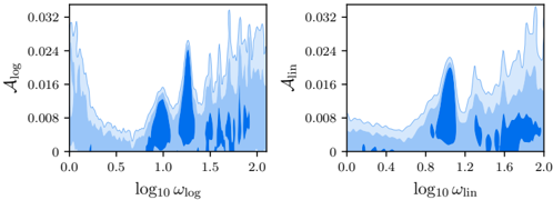
Fig. 22 Free-form Bayesian search for features (Sect. 6.2.2) with Planck TT,TE,EE + lowE + lensing. Upper panels : runs with linear priors on the k -locations. Lower panels : runs with logarithmic priors on the k -features. Left panels : reconstruction for N = 8 features. Right panels : reconstruction marginalized over N = 0 ; : : : ; 8 features.
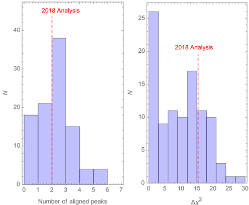
Fig. 22 Free-form Bayesian search for features (Sect. 6.2.2) with Planck TT,TE,EE + lowE + lensing. Upper panels : runs with linear priors on the k -locations. Lower panels : runs with logarithmic priors on the k -features. Left panels : reconstruction for N = 8 features. Right panels : reconstruction marginalized over N = 0 ; : : : ; 8 features.CC-BY · From the PDF
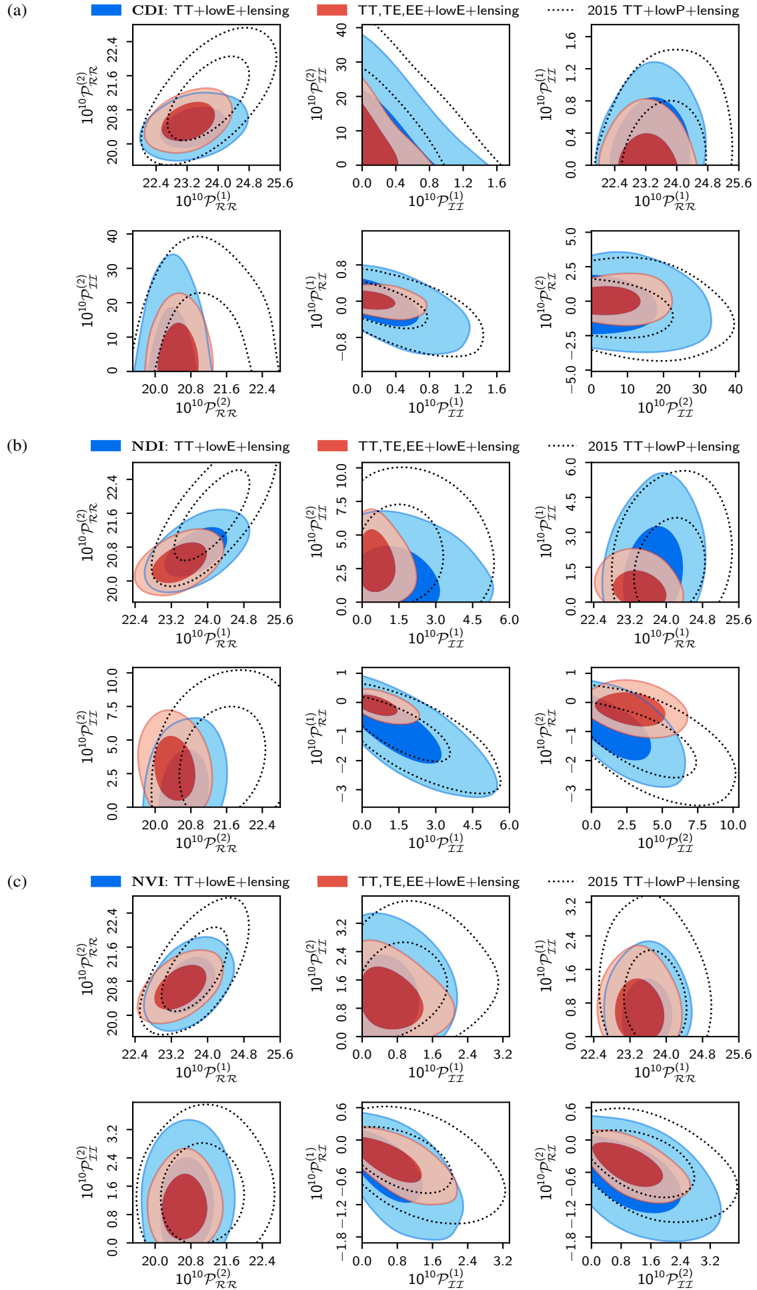
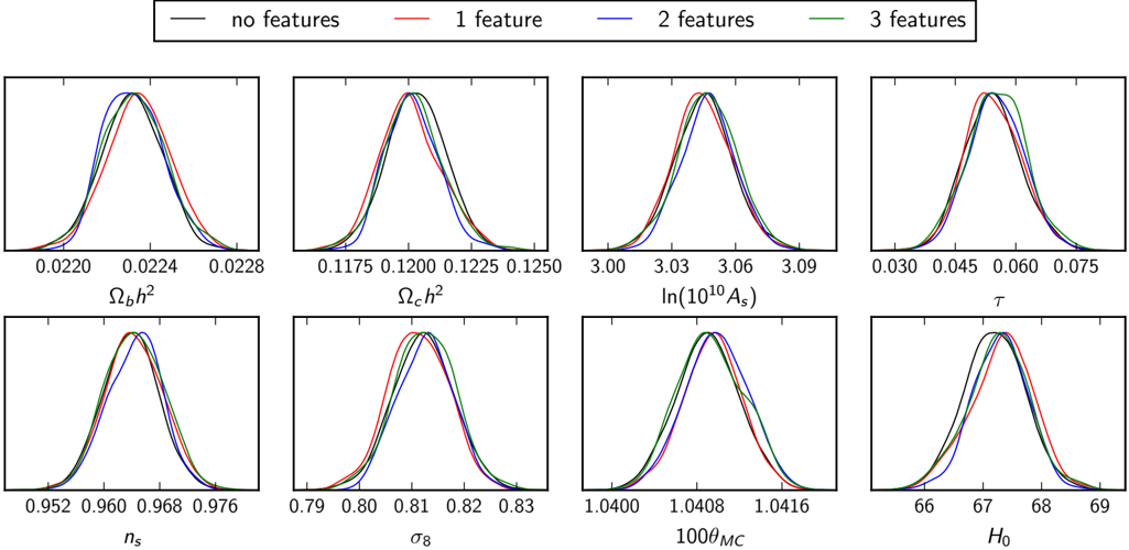
Fig. 23 E ect on the underlying cosmological parameters of the free-form Bayesian search for features (Sect. 6.2.2), for N = 0 ; : : : ; 3 features with linear k -priors. The parameters remain stable up to N = 8 features, and when changing to logarithmic k -priors.
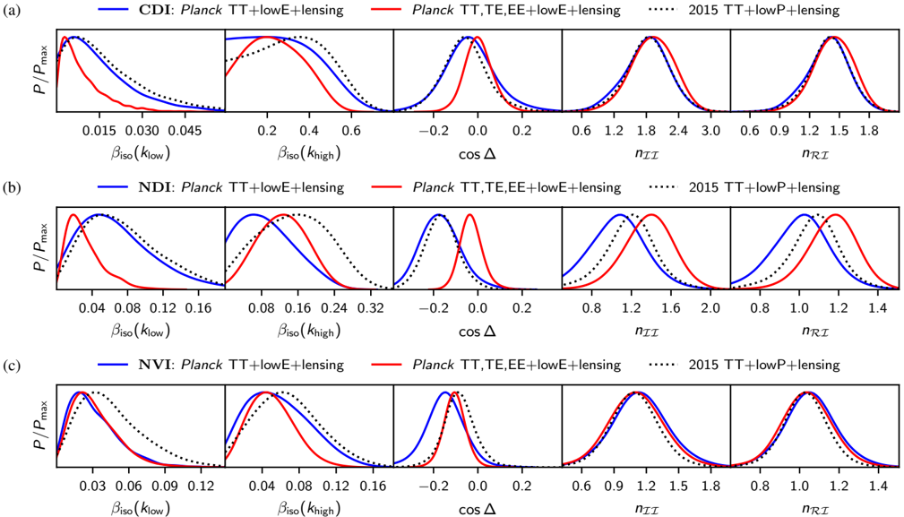
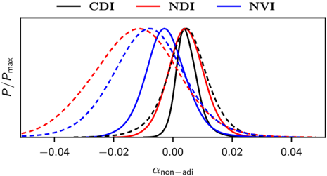
Fig. 23 E ect on the underlying cosmological parameters of the free-form Bayesian search for features (Sect. 6.2.2), for N = 0 ; : : : ; 3 features with linear k -priors. The parameters remain stable up to N = 8 features, and when changing to logarithmic k -priors.CC-BY · From the PDF
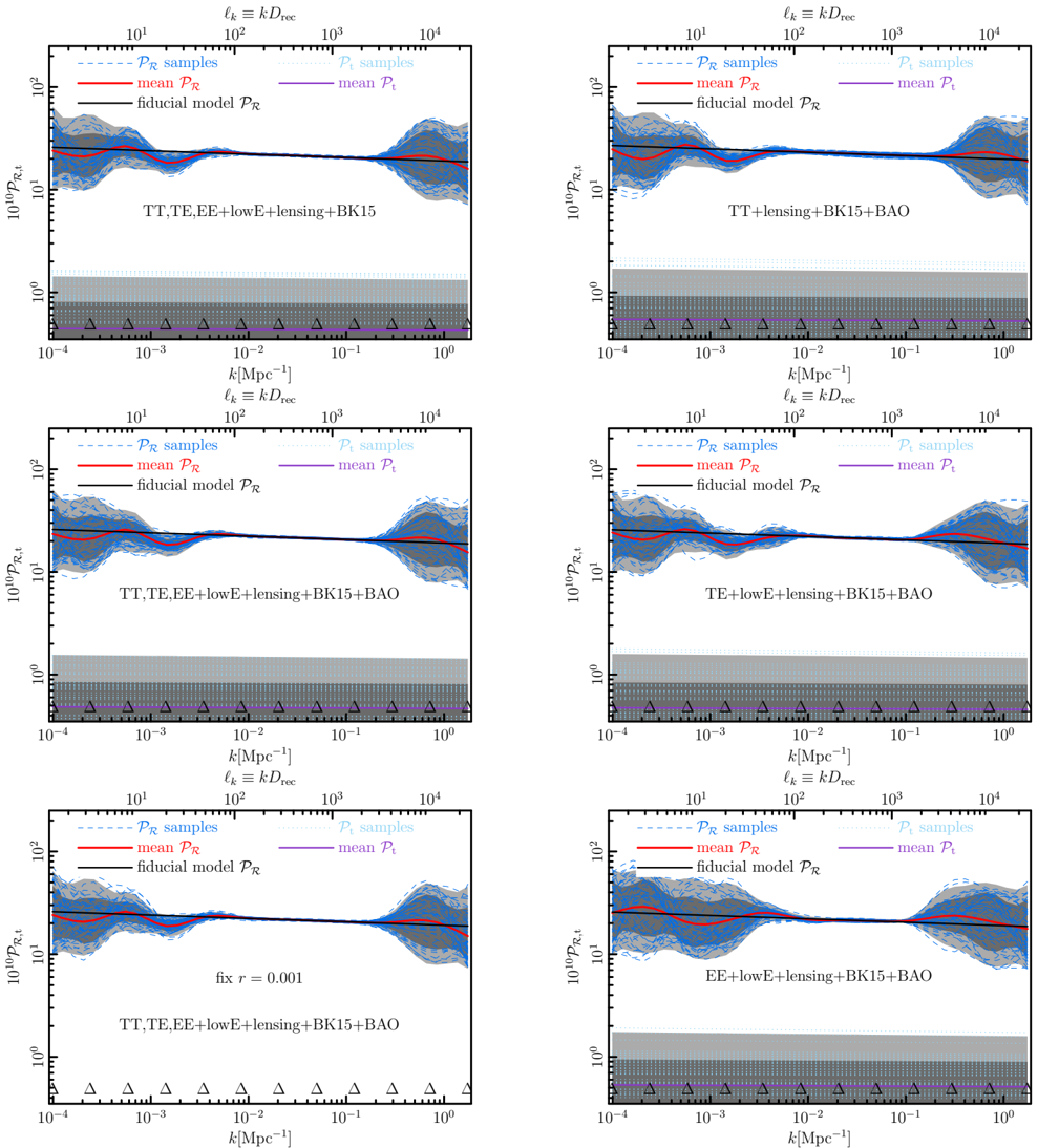
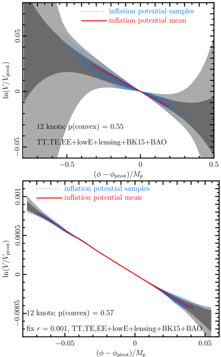
Fig. 24 Reconstructed primordial scalar power spectrum derived using Planck TT,TE,EE + lowE + lensing + BK15 data and 12 knots for the cubic spline interpolation (with positions marked as at the bottom of each panel). Mean (ensemble-averaged) spectra are heavy lines, allowed 1 and 2 regions for trajectories are the shaded regions, and the dashed lines denote selected trajectories with parameters sampled within the 1 posterior. Below the scalar power is the tensor power reconstruction. The addition of the BAO likelihood shown in the middle panel makes almost no visual di erence to the reconstructions. In the bottom panel , fixing the tensor-to-scalar ratio to r = 0 : 001 also produces only small di erences in reconstruction. Knot positions in k roughly translate to multipoles through kD rec , where D rec is the comoving distance to recombination.
Fig. 24 Reconstructed primordial scalar power spectrum derived using Planck TT,TE,EE + lowE + lensing + BK15 data and 12 knots for the cubic spline interpolation (with positions marked as at the bottom of each panel). Mean (ensemble-averaged) spectra are heavy lines, allowed 1 and 2 regions for trajectories are the shaded regions, and the dashed lines denote selected trajectories with parameters sampled within the 1 posterior. Below the scalar power is the tensor power reconstruction. The addition of the BAO likelihood shown in the middle panel makes almost no visual di erence to the reconstructions. In the bottom panel , fixing the tensor-to-scalar ratio to r = 0 : 001 also produces only small di erences in reconstruction. Knot positions in k roughly translate to multipoles through kD rec , where D rec is the comoving distance to recombination.CC-BY · From the PDF
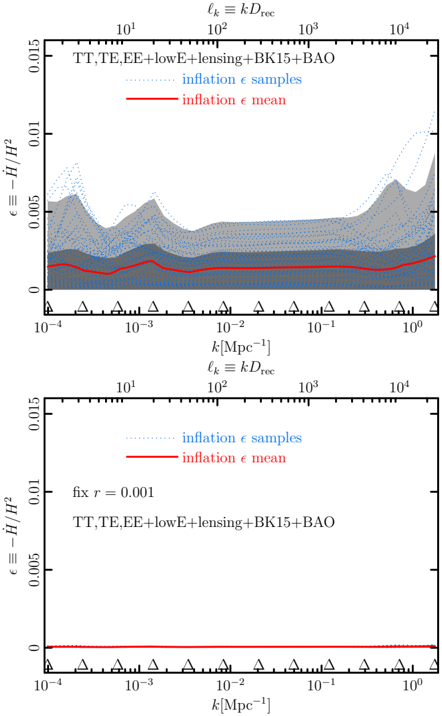
Fig. 26 Acceleration history ( k ) for reconstructed trajectories using 12 knots (marked as at the bottom of the figure), with cubic-spline interpolation and the Planck TT,TE,EE + lowE + lensing + BK15 + BAO data for the two cases of floating r and r fi xed at 0.001. Sample 1 trajectories for the floating r case allow wide variability, which is naturally greatly diminished if r is fixed to r = 0 : 001.
Fig. 26 Acceleration history ( k ) for reconstructed trajectories using 12 knots (marked as at the bottom of the figure), with cubic-spline interpolation and the Planck TT,TE,EE + lowE + lensing + BK15 + BAO data for the two cases of floating r and r fi xed at 0.001. Sample 1 trajectories for the floating r case allow wide variability, which is naturally greatly diminished if r is fixed to r = 0 : 001.CC-BY · From the PDF
Image 26
CC-BY · From the PDF
Image 27
CC-BY · From the PDF
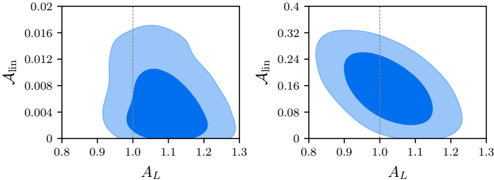
Fig. 29 Marginalized joint 68% and 95% CL regions for the lensing parameter A L and the modulation amplitude parameter A lin using the TT data set. Left: linear oscillation model with log 10 ! lin = 1 : 158 and ' lin = . Right: modified linear oscillation model with a Gaussian envelope function (see text) and log 10 ! lin = 1 : 158, ' lin = , env = 0 : 2 Mpc 1 , and env = 0 : 057 Mpc 1 :
Fig. 29 Marginalized joint 68% and 95% CL regions for the lensing parameter A L and the modulation amplitude parameter A lin using the TT data set. Left: linear oscillation model with log 10 ! lin = 1 : 158 and ' lin = . Right: modified linear oscillation model with a Gaussian envelope function (see text) and log 10 ! lin = 1 : 158, ' lin = , env = 0 : 2 Mpc 1 , and env = 0 : 057 Mpc 1 :CC-BY · From the PDF
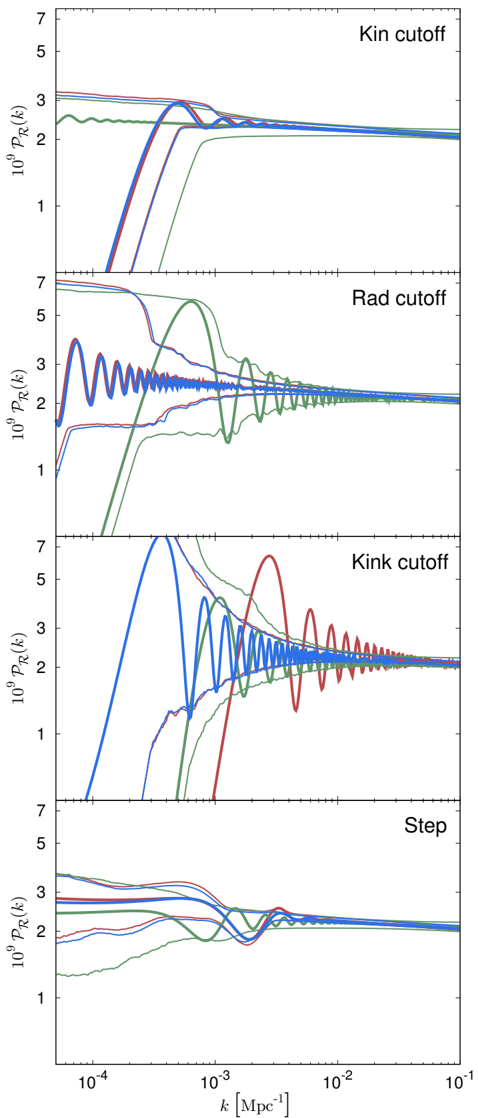
Fig. 30 Best-fit and central 95% CL regions for the primordial power spectrum in the three cuto and the step models for TT data (red curves), EE data (green), and TT,TE,EE data (blue). Note that for the combination of kink cuto model and TT data, the best-fit value for the cuto scale k c kink lies close to the prior boundary, and therefore the best-fit spectrum does not fall within the central 95%-credible band.
Fig. 30 Best-fit and central 95% CL regions for the primordial power spectrum in the three cuto and the step models for TT data (red curves), EE data (green), and TT,TE,EE data (blue). Note that for the combination of kink cuto model and TT data, the best-fit value for the cuto scale k c kink lies close to the prior boundary, and therefore the best-fit spectrum does not fall within the central 95%-credible band.CC-BY · From the PDF
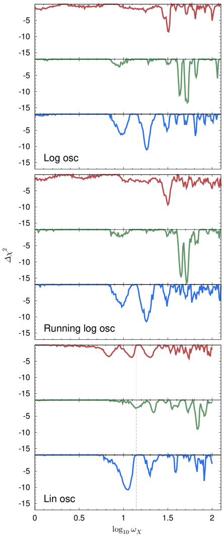
Fig. 31 Profile likelihood of the frequency parameter in the three oscillatory feature models for TT (red curves), EE (green), and TT,TE,EE data (blue). The dotted grey line in the bottom panels marks the frequency for which the linear oscillation model leads to a modulation of the angular power spectra whose wavelength roughly matches that of the CMB's acoustic oscillations. Note the lack of alignment between the temperature and polarization likelihood peaks in the vicinity of this frequency.
Fig. 31 Profile likelihood of the frequency parameter in the three oscillatory feature models for TT (red curves), EE (green), and TT,TE,EE data (blue). The dotted grey line in the bottom panels marks the frequency for which the linear oscillation model leads to a modulation of the angular power spectra whose wavelength roughly matches that of the CMB's acoustic oscillations. Note the lack of alignment between the temperature and polarization likelihood peaks in the vicinity of this frequency.CC-BY · From the PDF
Image 31
CC-BY · From the PDF
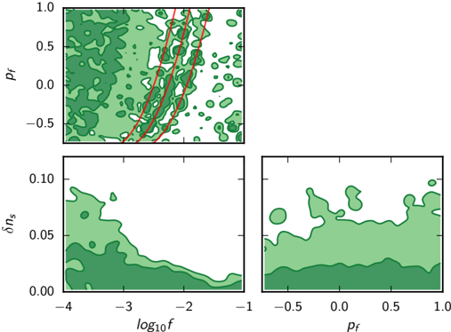
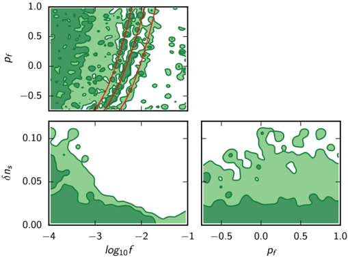
Fig. 33 Same as Fig. 32, but for the case of p = 1.
Fig. 33 Same as Fig. 32, but for the case of p = 1.CC-BY · From the PDF
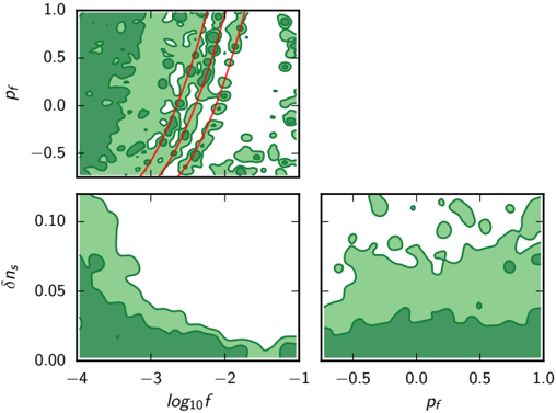
Fig. 34 Same as Fig. 32, but for the case of p = 2 = 3.
Fig. 34 Same as Fig. 32, but for the case of p = 2 = 3.CC-BY · From the PDF
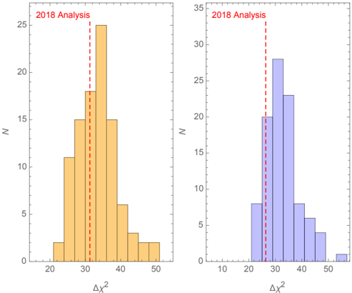
Fig. 35 Typical best-fit improvement in units of 2 in 100 simulations compared to the real data (red dashed lines) for the log feature ( left ) and the linear feature ( right ) models.
Fig. 35 Typical best-fit improvement in units of 2 in 100 simulations compared to the real data (red dashed lines) for the log feature ( left ) and the linear feature ( right ) models.CC-BY · From the PDF
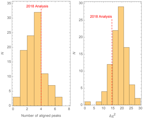
Fig. 36 Left : number of aligned peaks in the power spectrum and the bispectrum for the log feature model. Right : mean improvement of those same peaks in 100 simulated bispectra combined with the unbinned high-' likelihood.
Fig. 36 Left : number of aligned peaks in the power spectrum and the bispectrum for the log feature model. Right : mean improvement of those same peaks in 100 simulated bispectra combined with the unbinned high-' likelihood.CC-BY · From the PDF
Fig. 37 Left : number of aligned peaks in the power spectrum and the bispectrum for the linear feature model. Right : mean improvement of those same peaks in 100 simulated bispectra combined with the unbinned high-' likelihood.
Fig. 37 Left : number of aligned peaks in the power spectrum and the bispectrum for the linear feature model. Right : mean improvement of those same peaks in 100 simulated bispectra combined with the unbinned high-' likelihood.CC-BY · From the PDF
Image 37
CC-BY · From the PDF
Image 38
CC-BY · From the PDF
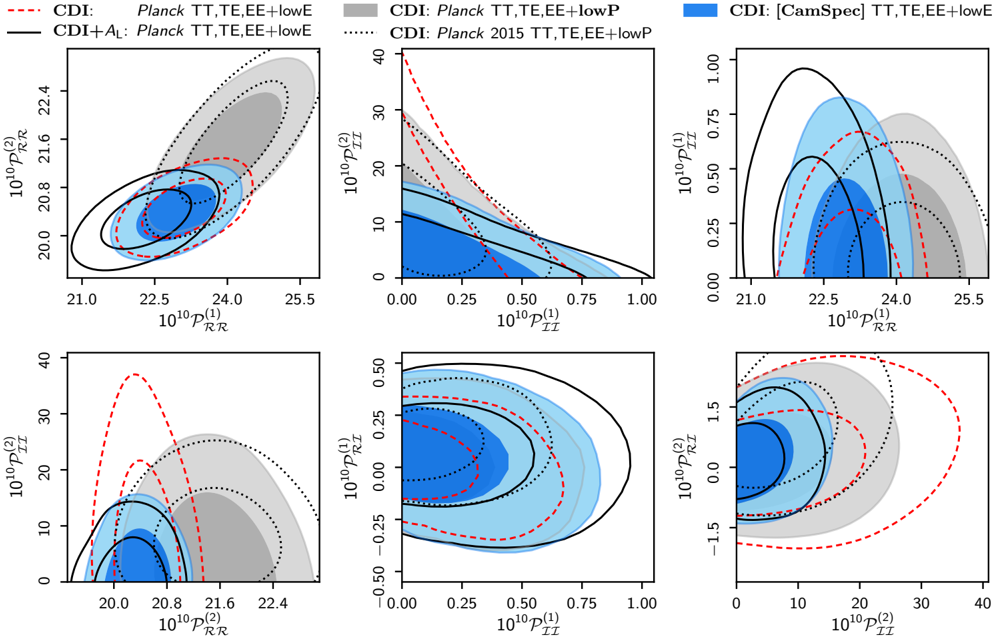
Fig. 39 Constraints on the primordial isocurvature fraction, iso , at k low = 0 : 002 Mpc 1 and k high = 0 : 100 Mpc 1 ; the primordial correlation fraction, cos ; the isocurvature spectral index, n II ; and the correlation spectral index, n RI = ( n RR + n II ) = 2, for the generally correlated mixed ADI + CDI model ( a ), for the ADI + NDI model ( b ), and for the ADI + NVI model ( c ). All these parameters are derived, and the distributions shown here result from a uniform prior on the primary parameters shown in Fig. 38. However, the e ect of the non-flat derived-parameter priors is negligible for all parameters except for n II (and n RI ) where the prior biases the distribution toward unity. Note that these spectral indices are not well constrained, since we do not have a detection of non-zero isocurvature or correlation amplitude. With a su ciently small isocurvature or correlation amplitude, an arbitrarily small or large spectral index leads to a very good fit to the data, since the model is then practically adiabatic over the range covered by the Planck data.
Fig. 39 Constraints on the primordial isocurvature fraction, iso , at k low = 0 : 002 Mpc 1 and k high = 0 : 100 Mpc 1 ; the primordial correlation fraction, cos ; the isocurvature spectral index, n II ; and the correlation spectral index, n RI = ( n RR + n II ) = 2, for the generally correlated mixed ADI + CDI model ( a ), for the ADI + NDI model ( b ), and for the ADI + NVI model ( c ). All these parameters are derived, and the distributions shown here result from a uniform prior on the primary parameters shown in Fig. 38. However, the e ect of the non-flat derived-parameter priors is negligible for all parameters except for n II (and n RI ) where the prior biases the distribution toward unity. Note that these spectral indices are not well constrained, since we do not have a detection of non-zero isocurvature or correlation amplitude. With a su ciently small isocurvature or correlation amplitude, an arbitrarily small or large spectral index leads to a very good fit to the data, since the model is then practically adiabatic over the range covered by the Planck data.CC-BY · From the PDF
Image 40
CC-BY · From the PDF
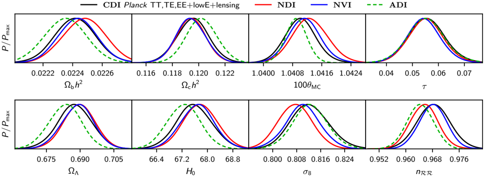
Fig. 41 Comparison of the posterior probability density for the standard cosmological parameters in mixed adiabatic and isocurvature models (solid lines) to those in the pure adiabatic CDMmodel (ADI, dashed green lines), using Planck TT,TE,EE + lowE + lensing data.
Fig. 41 Comparison of the posterior probability density for the standard cosmological parameters in mixed adiabatic and isocurvature models (solid lines) to those in the pure adiabatic CDMmodel (ADI, dashed green lines), using Planck TT,TE,EE + lowE + lensing data.CC-BY · From the PDF
Image 42
CC-BY · From the PDF
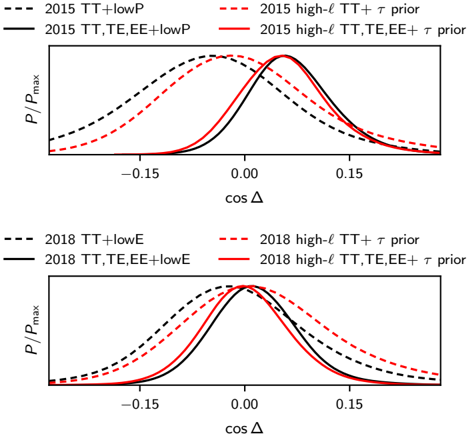
Fig. 44 Scale-independent primordial correlation fraction in the mixed adiabatic and CDI model. The black curves are with Planck high-' and low-' data, while the red ones result from using only the high-' Plik likelihood supplemented with a Gaussian prior on the optical depth. For the 2015 data ( top panel ) this prior was = 0 : 078 0 : 019, whereas for the 2018 case ( bottom panel ) we have adopted = 0 : 055 0 : 007 from the Planck 2018 TT,TE,EE + lowE + lensing CDI chain.
Fig. 44 Scale-independent primordial correlation fraction in the mixed adiabatic and CDI model. The black curves are with Planck high-' and low-' data, while the red ones result from using only the high-' Plik likelihood supplemented with a Gaussian prior on the optical depth. For the 2015 data ( top panel ) this prior was = 0 : 078 0 : 019, whereas for the 2018 case ( bottom panel ) we have adopted = 0 : 055 0 : 007 from the Planck 2018 TT,TE,EE + lowE + lensing CDI chain.CC-BY · From the PDF
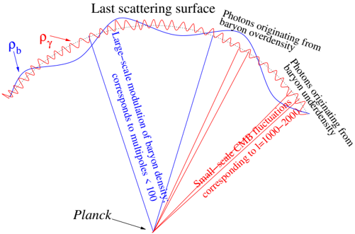
Fig. 45 Illustration of how the large-scale modulation of the baryon density by CIP gets converted into a small-scale 'smoothing' e ect of the temperature and polarization anisotropies.
Fig. 45 Illustration of how the large-scale modulation of the baryon density by CIP gets converted into a small-scale 'smoothing' e ect of the temperature and polarization anisotropies.CC-BY · From the PDF
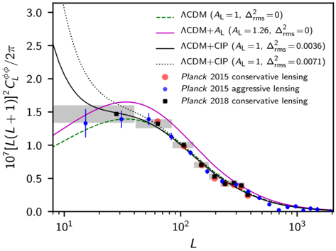
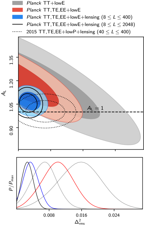
Fig. 46 Conservative Planck 2015 lensing data (red points), aggressive Planck 2015 lensing data (blue points with error bars), and conservative Planck 2018 lensing data (black squares in grey boxes), along with the best-fit models to the Planck data: the best-fit adiabatic CDM model to 2018 TT + lowE (green dashed line); the best-fit CDM + A L model to 2018 TT + lowE (magenta solid line, A L = 1 : 26); and the best-fit CDM + CIP model to 2018 TT,TE,EE + lowE and conservative lensing data (black solid line, 2 rms = 0 : 0036) and to 2015 TT,TE,EE + lowP and conservative lensing data (black dotted line, 2 rms = 0 : 0071). As CIP modifies only the very lowL part of the lensing power spectrum, the conservative 2015 lensing data (40 L 400) are insensitive to CIP even when 2 rms = 0 : 0071. On the other hand, the first two data points of the 2015 aggressive lensing data disfavour the large CIP amplitude (Smith et al. 2017), which gives a very good fit to all the other data. Planck 2018 conservative lensing data cover the range 8 L 400 and consequently disfavour CIP variances 2 rms & 0 : 004.
Fig. 46 Conservative Planck 2015 lensing data (red points), aggressive Planck 2015 lensing data (blue points with error bars), and conservative Planck 2018 lensing data (black squares in grey boxes), along with the best-fit models to the Planck data: the best-fit adiabatic CDM model to 2018 TT + lowE (green dashed line); the best-fit CDM + A L model to 2018 TT + lowE (magenta solid line, A L = 1 : 26); and the best-fit CDM + CIP model to 2018 TT,TE,EE + lowE and conservative lensing data (black solid line, 2 rms = 0 : 0036) and to 2015 TT,TE,EE + lowP and conservative lensing data (black dotted line, 2 rms = 0 : 0071). As CIP modifies only the very lowL part of the lensing power spectrum, the conservative 2015 lensing data (40 L 400) are insensitive to CIP even when 2 rms = 0 : 0071. On the other hand, the first two data points of the 2015 aggressive lensing data disfavour the large CIP amplitude (Smith et al. 2017), which gives a very good fit to all the other data. Planck 2018 conservative lensing data cover the range 8 L 400 and consequently disfavour CIP variances 2 rms & 0 : 004.CC-BY · From the PDF
Fig. 47 Degeneracy between A L and 2 rms in the CDM + A L + CIP model ( top panel ) and constraints on 2 rms in the CDM + CIP model, where A L = 1 ( bottom panel ).
Fig. 47 Degeneracy between A L and 2 rms in the CDM + A L + CIP model ( top panel ) and constraints on 2 rms in the CDM + CIP model, where A L = 1 ( bottom panel ).CC-BY · From the PDF
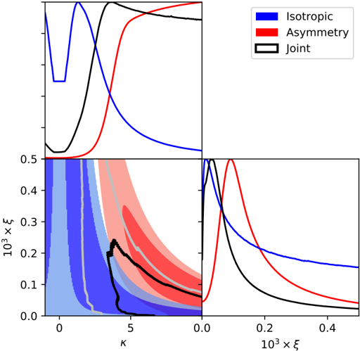
Fig. 48 Posteriors for the curvaton dipolar modulation model parameters and . Contours enclose 68% and 95% of the posteriors. The model can explain the well-known dipolar asymmetry: note the preference for > 0 in the asymmetry constraint (red contours and curves). However, the modulation preferred by the asymmetry constraint is reduced substantially when the isotropic constraint (blue) is added (black). The asymmetry constraint here uses SMICA , while the isotropic constraint uses Planck TT,TE,EE + lowE + lensing. Resolution is reduced at very small due to the sampling in iso .
Fig. 48 Posteriors for the curvaton dipolar modulation model parameters and . Contours enclose 68% and 95% of the posteriors. The model can explain the well-known dipolar asymmetry: note the preference for > 0 in the asymmetry constraint (red contours and curves). However, the modulation preferred by the asymmetry constraint is reduced substantially when the isotropic constraint (blue) is added (black). The asymmetry constraint here uses SMICA , while the isotropic constraint uses Planck TT,TE,EE + lowE + lensing. Resolution is reduced at very small due to the sampling in iso .CC-BY · From the PDF
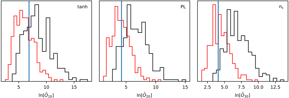
Fig. 49 Histograms of the quantity ˆ Oj 0 for the tanh, power-law, and n s gradient modulation models using Planck temperature data combined with 300 statistically isotropic polarization simulations (red outlines) or 300 polarization simulations modulated according to the best-fit parameters from the temperature data (black). The blue lines indicate the values for the actual SMICA polarization data. A large value relative to the isotropic (red) simulations would indicate that the modulation model is preferred over CDM.
Fig. 49 Histograms of the quantity ˆ Oj 0 for the tanh, power-law, and n s gradient modulation models using Planck temperature data combined with 300 statistically isotropic polarization simulations (red outlines) or 300 polarization simulations modulated according to the best-fit parameters from the temperature data (black). The blue lines indicate the values for the actual SMICA polarization data. A large value relative to the isotropic (red) simulations would indicate that the modulation model is preferred over CDM.CC-BY · From the PDF
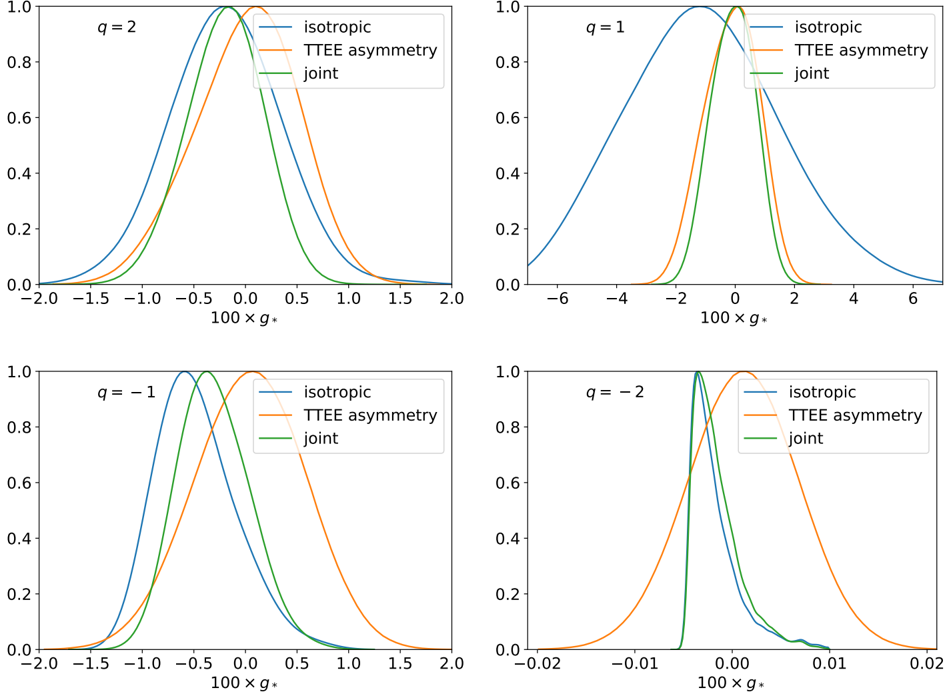
Fig. 50 Marginalized posteriors for quadrupolar modulation parameter g , using SMICA data for the TT + EE asymmetry constraints (orange curves) and Planck TT,TE,EE + lowE for the isotropic constraints (blue curves), which probe the modification to the power spectrum via Eq. (114). Top : constraints for q = 2 and 1 ( left and right , respectively). Bottom : constraints for q = 1 and 2 ( left and right , respectively). Strongly negative g is suppressed for q < 0, due to the unphysical prediction of negative power.
Fig. 50 Marginalized posteriors for quadrupolar modulation parameter g , using SMICA data for the TT + EE asymmetry constraints (orange curves) and Planck TT,TE,EE + lowE for the isotropic constraints (blue curves), which probe the modification to the power spectrum via Eq. (114). Top : constraints for q = 2 and 1 ( left and right , respectively). Bottom : constraints for q = 1 and 2 ( left and right , respectively). Strongly negative g is suppressed for q < 0, due to the unphysical prediction of negative power.CC-BY · From the PDF

Verification

Claims the paper makes

The claims and statistics of this paper haven’t been checked yet.

Run the check — free, no account needed. It reads the open-access text and checks the sources it cites.

A few free checks a day · papers already verified open instantly · results are public

Claims other papers make about this one

Each is checked against this paper’s own text: does it say what the citing paper says it does?

Self-check

Percentages, sums and reported differences re-computed from the paper’s own numbers.

The self-check needs the paper’s full text.

Citations

Cites

Show all 305 references

Research works printed but not linked: 19

  1. Audren, 2013, JCAP, 1302, 001
  2. Bennett, 2012, ApJS, 208, 54
  3. Bozza, 2003, JCAP, 0305, 001
  4. Dvali G., Shafi Q., & Solganik S. 2001, [arXiv:hep-th/0105203] · arXiv
  5. Easther, 2005, JCAP, 0505, 009
  6. Efstathiou G., & Gratton S. 2019, ArXiv e-prints [arXiv:1910.00483] · arXiv
  7. Goncharov, 1984, Sov. Phys. JETP, 59, 930
  8. Gong, 2001, Phys. Lett. B, 510, 1
  9. Haslam, 1982, A&AS, 47, 1
  10. Linde A. 2015, Proceedings, 100th Les Houches Summer School: Post-Planck Cosmology: Les Houches, France, July 8–August 2, 2013, 231
  11. Martin, 2014, JCAP, 1403, 039
  12. Mukhanov, 1985, JETP Lett., 41, 493
  13. Mukhanov, 1981, JETP Lett., 33, 532
  14. Mukhanov, 1982, Sov. Phys. JETP, 56, 258
  15. Planck Collaboration X, 2020, A&A, 641, A10, 10.1051/0004-6361/201833887
  16. Skilling J. 2004, in AIP Conf. Ser., eds. Fischer R., Preuss R., & Toussaint U. V., 735, 395
  17. Starobinsky, 1983, Sov. Astron. Lett., 9, 302
  18. Starobinsky, 1992, JETP Lett., 55, 489
  19. Waterhouse T. P., & Zibin J. P. 2008, ArXiv e-prints [arXiv:0804.1771] · arXiv

Cited by

See all 2,442

Metadata

Authors
Planck Collaboration, Akrami, Y., Arroja, F., Ashdown, M., Aumont, J., Baccigalupi, C., Ballardini, M., Banday, A. J., Barreiro, R. B., Bartolo, N., Basak, S., Benabed, K., Bernard, J.-P., Bersanelli, M., Bielewicz, P., Bock, J. J., Bond, J. R., Borrill, J., Bouchet, F. R., Boulanger, F., Bucher, M., Burigana, C., Butler, R. C., Calabrese, E., Cardoso, J.-F., Carron, J., Challinor, A., Chiang, H. C., Colombo, L. P. L., Combet, C., Contreras, D., Crill, B. P., Cuttaia, F., de Bernardis, P., de Zotti, G., Delabrouille, J., Delouis, J.-M., Di Valentino, E., Diego, J. M., Donzelli, S., Doré, O., Douspis, M., Ducout, A., Dupac, X., Dusini, S., Efstathiou, G., Elsner, F., Enßlin, T. A., Eriksen, H. K., Fantaye, Y., Fergusson, J., Fernandez-Cobos, R., Finelli, F., Forastieri, F., Frailis, M., Franceschi, E., Frolov, A., Galeotta, S., Galli, S., Ganga, K., Gauthier, C., Génova-Santos, R. T., Gerbino, M., Ghosh, T., González-Nuevo, J., Górski, K. M., Gratton, S., Gruppuso, A., Gudmundsson, J. E., Hamann, J., Handley, W., Hansen, F. K., Herranz, D., Hivon, E., Hooper, D. C., Huang, Z., Jaffe, A. H., Jones, W. C., Keihänen, E., Keskitalo, R., Kiiveri, K., Kim, J., Kisner, T. S., Krachmalnicoff, N., Kunz, M., Kurki-Suonio, H., Lagache, G., Lamarre, J.-M., Lasenby, A., Lattanzi, M., Lawrence, C. R., Le Jeune, M., Lesgourgues, J., Levrier, F., Lewis, A., Liguori, M., Lilje, P. B., Lindholm, V., López-Caniego, M., Lubin, P. M., Ma, Y.-Z., Macías-Pérez, J. F., Maggio, G., Maino, D., Mandolesi, N., Mangilli, A., Marcos-Caballero, A., Maris, M., Martin, P. G., Martínez-González, E., Matarrese, S., Mauri, N., McEwen, J. D., Meerburg, P. D., Meinhold, P. R., Melchiorri, A., Mennella, A., Migliaccio, M., Mitra, S., Miville-Deschênes, M.-A., Molinari, D., Moneti, A., Montier, L., Morgante, G., Moss, A., Münchmeyer, M., Natoli, P., Nørgaard-Nielsen, H. U., Pagano, L., Paoletti, D., Partridge, B., Patanchon, G., Peiris, H. V., Perrotta, F., Pettorino, V., Piacentini, F., Polastri, L., Polenta, G., Puget, J.-L., Rachen, J. P., Reinecke, M., Remazeilles, M., Renzi, A., Rocha, G., Rosset, C., Roudier, G., Rubiño-Martín, J. A., Ruiz-Granados, B., Salvati, L., Sandri, M., Savelainen, M., Scott, D., Shellard, E. P. S., Shiraishi, M., Sirignano, C., Sirri, G., Spencer, L. D., Sunyaev, R., Suur-Uski, A.-S., Tauber, J. A., Tavagnacco, D., Tenti, M., Toffolatti, L., Tomasi, M., Trombetti, T., Valiviita, J., Van Tent, B., Vielva, P., Villa, F., Vittorio, N., Wandelt, B. D., Wehus, I. K., White, S. D. M., Zacchei, A., Zibin, J. P., & Zonca, A.
Venue
Astronomy & Astrophysics
Publisher
EDP Sciences
Published
2020-09
Volume
641
Pages
A10
ISSN
  • 0004-6361
  • 1432-0746
Cited by
2,442
References
305

About these checks

Registry, retraction, Cites and statistics results are computed, not judged, with one exception: a printed reference that no index lists is read once by a model before it counts as a citation error. Claims are extracted by a model and kept only when their quote appears verbatim in the text; each cited source is then checked, with a model’s help, for whether it says what the claim relies on. Those verdicts can be wrong — read the claim’s quote and the cited source before relying on one.

Statistics and arithmetic are recomputed, not judged.

Confidence bands are shown only for fields calibrated on our annotated test set. None is calibrated yet, so no band is shown.

What counts as a claim ›How we measure confidence ›How we check this ›

Are you an author, or do you see a problem with this page? Request a review

How to cite

Cite CoChat for the checks on this page, and the paper for its own findings.

This page
CoChat. (2026). Citation check: Planck 2018 results: X. Constraints on inflation. https://app.cochat.ai/papers/10.1051/0004-6361/201833887
The paper
Planck Collaboration, Akrami, Y., Arroja, F., Ashdown, M., Aumont, J., Baccigalupi, C., Ballardini, M., Banday, A. J., Barreiro, R. B., Bartolo, N., Basak, S., Benabed, K., Bernard, J.-P., Bersanelli, M., Bielewicz, P., Bock, J. J., Bond, J. R., Borrill, J., Bouchet, F. R., . . . Zonca, A. (2020). Planck 2018 results: X. Constraints on inflation. Astronomy & Astrophysics. https://doi.org/10.1051/0004-6361/201833887

Data sources

Bibliographic data: Semantic Scholar, OpenAlex, Crossref.

Contains information from the Semantic Scholar Academic Graph Datasets, made available under the ODC Attribution License (ODC-BY 1.0).

Semantic Scholar’s data is described in: Kinney, R., et al. (2023). The Semantic Scholar Open Data Platform. arXiv:2301.10140.