Cited by 303

The DOI matches its Crossref record; 7 of the 7 references it cites were found in a registry or an index.

Two-dimensionally confined topological edge states in photonic crystals

Barik, Sabyasachi, Miyake, Hirokazu, DeGottardi, Wade, Waks, Edo, Hafezi, Mohammad·2016·New Journal of Physics

Overview

The claims and statistics of this paper haven’t been checked yet.

Run the check — free, no account needed. It reads the open-access text and checks the sources it cites.

A few free checks a day · papers already verified open instantly · results are public

Integrity signals

Registry

Crossref · 10.1088/1367-2630/18/11/113013

Cites

7 of 7 references verified0 citation errors · 0 not checkable

Statistics

Figures

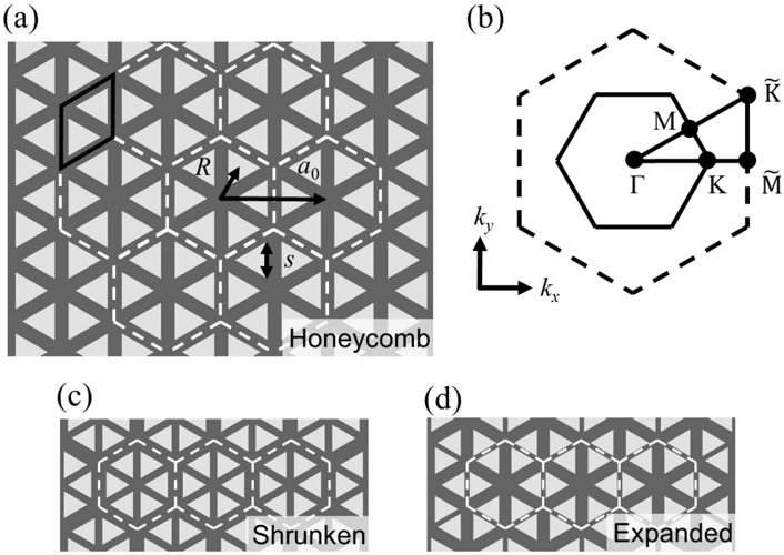
Figure 1 Schematic of our proposed honeycomb-lattice-like photonic crystal. (a) Baseline structure of equilateral triangular holes arranged in a honeycomb lattice in a dielectric material. This honeycomb lattice can be viewed as a triangular lattice of two-hole unit cells (black solid rhombus), or alternatively as a triangular lattice of six-hole unit cells (white dashed hexagons), which we call honeycomb clusters with R = a 0 / 3. (b) First Brillouin zones for the six-hole (solid) and two-hole (dashed) unit cells. The letters indicate high-symmetry points. (c) [and (d)] Same structure as in (a) except that R < a 0 / 3 ( R > a 0 / 3), which we call shrunken (expanded) clusters.
Figure 1 Schematic of our proposed honeycomb-lattice-like photonic crystal. (a) Baseline structure of equilateral triangular holes arranged in a honeycomb lattice in a dielectric material. This honeycomb lattice can be viewed as a triangular lattice of two-hole unit cells (black solid rhombus), or alternatively as a triangular lattice of six-hole unit cells (white dashed hexagons), which we call honeycomb clusters with R = a 0 / 3. (b) First Brillouin zones for the six-hole (solid) and two-hole (dashed) unit cells. The letters indicate high-symmetry points. (c) [and (d)] Same structure as in (a) except that R < a 0 / 3 ( R > a 0 / 3), which we call shrunken (expanded) clusters.CC-BY · From the PDF
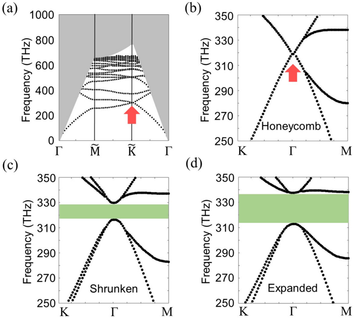
Figure 2 Band structures show opening and closing of a band gap around the Dirac point as we perturb the lattice. (a) Band structure of the honeycomb lattice in the two-hole unit cell picture. The gray area represents the region above the light line, where light can leak out of the plane. A Dirac point exists at the ˜ K point (red arrow) and is below the light line. (b),(c) and (d) Band structure calculated with the six-hole unit cell with honeycomb clusters ( R = a 0 / 3), shrunken clusters ( R = 0 . 91 × a 0 / 3), and expanded clusters ( R = 1 . 09 × a 0 / 3) respectively. The red arrow indicates the Dirac point, and the green areas represent the band gap.
Figure 2 Band structures show opening and closing of a band gap around the Dirac point as we perturb the lattice. (a) Band structure of the honeycomb lattice in the two-hole unit cell picture. The gray area represents the region above the light line, where light can leak out of the plane. A Dirac point exists at the ˜ K point (red arrow) and is below the light line. (b),(c) and (d) Band structure calculated with the six-hole unit cell with honeycomb clusters ( R = a 0 / 3), shrunken clusters ( R = 0 . 91 × a 0 / 3), and expanded clusters ( R = 1 . 09 × a 0 / 3) respectively. The red arrow indicates the Dirac point, and the green areas represent the band gap.CC-BY · From the PDF
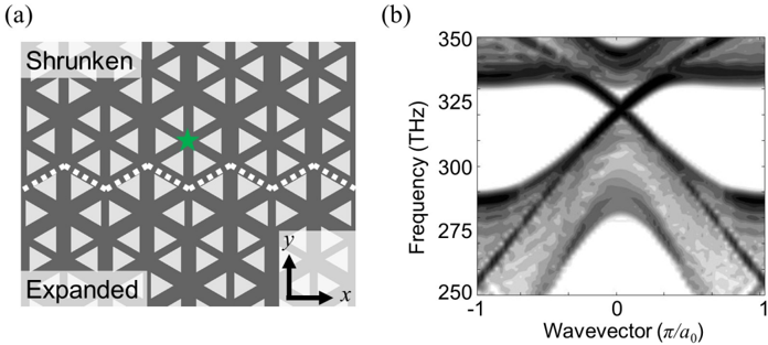
Figure 3 Schematic and band structure which gives rise to topological edge states. (a) Schematic of two regions with different band topologies. White dotted line marks the boundary between the two regions. The star (green) indicates the location where we placed a circularly-polarized electric dipole to excite topological edge states. (b) Corresponding one-dimensional band structure shows two bands crossing the band gap in bulk. The opposite group velocities in the crossing region indicate the existence of counter-propagating directional edge states.
Figure 3 Schematic and band structure which gives rise to topological edge states. (a) Schematic of two regions with different band topologies. White dotted line marks the boundary between the two regions. The star (green) indicates the location where we placed a circularly-polarized electric dipole to excite topological edge states. (b) Corresponding one-dimensional band structure shows two bands crossing the band gap in bulk. The opposite group velocities in the crossing region indicate the existence of counter-propagating directional edge states.CC-BY · From the PDF
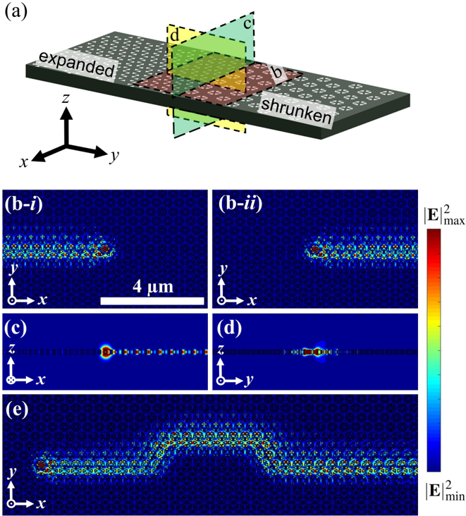
Figure 4 Three-dimensional, vertically-confined topological edge states at optical frequencies in an all-dielectric material. (a) Schematic diagram of the threedimensional photonic crystal where the colored planes correspond to the cross-sections shown in (b), (c), and (d). (bi ) and (bii ) Electric field intensities for a topological edge state excited with a positively and negatively circularly-polarized electric dipole show directional propagation in the -x and + x directions respectively. (c) and (d) Cross-section view along the xz and yz plane of the electric field intensity confirms that total internal reflection at the air-dielectric boundary prevents light from leaking out of the plane. (e) Electric field intensity for an edge state with four 90 ◦ bends show that light can propagate around defects without backscattering.
Figure 4 Three-dimensional, vertically-confined topological edge states at optical frequencies in an all-dielectric material. (a) Schematic diagram of the threedimensional photonic crystal where the colored planes correspond to the cross-sections shown in (b), (c), and (d). (bi ) and (bii ) Electric field intensities for a topological edge state excited with a positively and negatively circularly-polarized electric dipole show directional propagation in the -x and + x directions respectively. (c) and (d) Cross-section view along the xz and yz plane of the electric field intensity confirms that total internal reflection at the air-dielectric boundary prevents light from leaking out of the plane. (e) Electric field intensity for an edge state with four 90 ◦ bends show that light can propagate around defects without backscattering.CC-BY · From the PDF
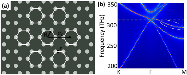
Figure 5 Band structure of a honeycomb lattice with circular holes. (a) Schematic of a honeycomb lattice made of circular holes, where the parameters a 0 is the lattice constant of the hexagonal clusters (white hexagons) which constitute a triangular lattice, R is the distance from the center of the cluster to the center of a circular hole within the cluster ( R = a 0 / 3 in this case), and s is the diameter of the circular hole. (b) Band structure for transverse-electric modes of the structure shown in (a), showing the appearance of a Dirac cone at 312 THz (indicated by the horizontal white dashed line). White dotted ellipse shows one of the bands crossing the frequency at the Dirac point, which prevents the appearance of a band gap across the Brillouin zone after perturbation. Calculations were done with a 0 = 350 nm and s = 140 nm.
Figure 5 Band structure of a honeycomb lattice with circular holes. (a) Schematic of a honeycomb lattice made of circular holes, where the parameters a 0 is the lattice constant of the hexagonal clusters (white hexagons) which constitute a triangular lattice, R is the distance from the center of the cluster to the center of a circular hole within the cluster ( R = a 0 / 3 in this case), and s is the diameter of the circular hole. (b) Band structure for transverse-electric modes of the structure shown in (a), showing the appearance of a Dirac cone at 312 THz (indicated by the horizontal white dashed line). White dotted ellipse shows one of the bands crossing the frequency at the Dirac point, which prevents the appearance of a band gap across the Brillouin zone after perturbation. Calculations were done with a 0 = 350 nm and s = 140 nm.CC-BY · From the PDF
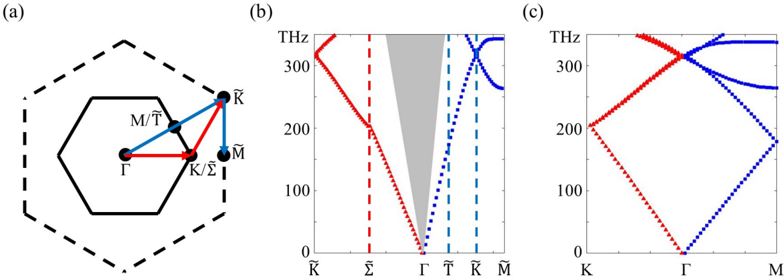
Figure 6 Correspondence between the two-site and six-site bases. (a) Boundaries of the first Brillouin zone for the two-site (dashed hexagon) and six-site (solid hexagon) bases for the honeycomb lattice. (b) The band structure of the honeycomb lattice considered with a two-site basis. The labels on the horizontal axis corresponds to the high-symmetry points in k -space as designated in (a) [31]. The gray area is the area above the light cone where guided modes are not possible. The red triangles (blue squares) correspond to the red (blue) paths indicated in (a). (c) The band structure of the honeycomb lattice with a six-site basis as obtained by folding the band structure in (b) along the dotted vertical lines.
Figure 6 Correspondence between the two-site and six-site bases. (a) Boundaries of the first Brillouin zone for the two-site (dashed hexagon) and six-site (solid hexagon) bases for the honeycomb lattice. (b) The band structure of the honeycomb lattice considered with a two-site basis. The labels on the horizontal axis corresponds to the high-symmetry points in k -space as designated in (a) [31]. The gray area is the area above the light cone where guided modes are not possible. The red triangles (blue squares) correspond to the red (blue) paths indicated in (a). (c) The band structure of the honeycomb lattice with a six-site basis as obtained by folding the band structure in (b) along the dotted vertical lines.CC-BY · From the PDF
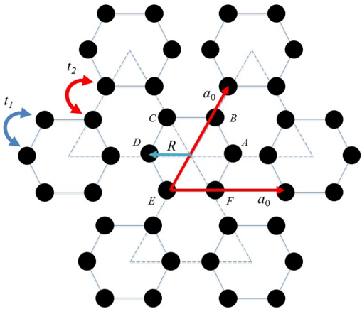
Figure 7 Schematic of our lattice parameters and the labeling of the lattice sites for our tight-binding model. A cluster consists of six sites. Then the system is a triangular lattice of clusters with lattice constant a 0 . The distance from the centroid of each hole to the center of its cluster is R . The tunneling amplitudes t 1 and t 2 correspond to intra- and inter-cluster tunneling between the nearest neighbor holes. The labels A, B, C, D, E, F denote each lattice site making up the basis.
Figure 7 Schematic of our lattice parameters and the labeling of the lattice sites for our tight-binding model. A cluster consists of six sites. Then the system is a triangular lattice of clusters with lattice constant a 0 . The distance from the centroid of each hole to the center of its cluster is R . The tunneling amplitudes t 1 and t 2 correspond to intra- and inter-cluster tunneling between the nearest neighbor holes. The labels A, B, C, D, E, F denote each lattice site making up the basis.CC-BY · From the PDF
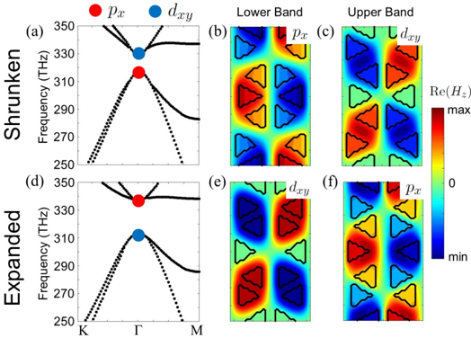
Figure 8 Band inversion. (a) and (d) Band structures for the shrunken and expanded cluster systems, which are the same as Fig. 2(c) and (d) respectively in the main text, with a subset of the eigenstates indicated at the Γ point. (b) and (c) [(e) and (f)] Out-of-plane magnetic field eigenstates at the symmetry plane z = 0 of the lower and upper band for the shrunken (expanded) cluster system respectively. We see that e.g. , the eigenstate p x for the lower band in the shrunken cluster system appears on the upper band for the expanded cluster system, which indicates a change in the band topology.
Figure 8 Band inversion. (a) and (d) Band structures for the shrunken and expanded cluster systems, which are the same as Fig. 2(c) and (d) respectively in the main text, with a subset of the eigenstates indicated at the Γ point. (b) and (c) [(e) and (f)] Out-of-plane magnetic field eigenstates at the symmetry plane z = 0 of the lower and upper band for the shrunken (expanded) cluster system respectively. We see that e.g. , the eigenstate p x for the lower band in the shrunken cluster system appears on the upper band for the expanded cluster system, which indicates a change in the band topology.CC-BY · From the PDF
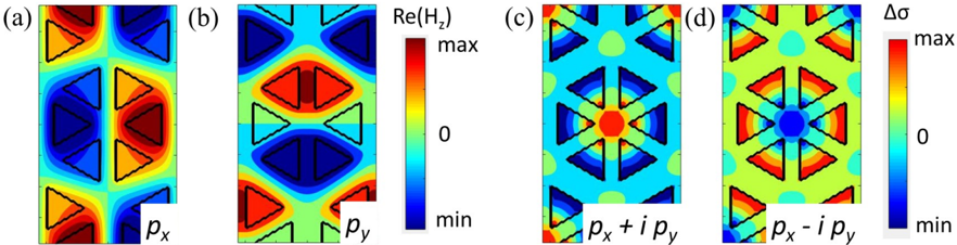
Figure 9 Out-of-plane magnetic field and in-plane electric field polarization in a cluster of six holes outlined by black triangles. (a) and (b) depict the real part of the out-of-plane magnetic field ( H z ) for the eigenstates p x and p y respectively. The colors indicate the strength of H z . (c) and (d) show ∆ σ ∼ | E + | 2 - | E -| 2 , indicating the pseudo-spin nature of the bands excited at the Γ point with p x + ip y and p x -ip y modes, respectively.
Figure 9 Out-of-plane magnetic field and in-plane electric field polarization in a cluster of six holes outlined by black triangles. (a) and (b) depict the real part of the out-of-plane magnetic field ( H z ) for the eigenstates p x and p y respectively. The colors indicate the strength of H z . (c) and (d) show ∆ σ ∼ | E + | 2 - | E -| 2 , indicating the pseudo-spin nature of the bands excited at the Γ point with p x + ip y and p x -ip y modes, respectively.CC-BY · From the PDF

Verification

Claims the paper makes

The claims and statistics of this paper haven’t been checked yet.

Run the check — free, no account needed. It reads the open-access text and checks the sources it cites.

A few free checks a day · papers already verified open instantly · results are public

Claims other papers make about this one

Each is checked against this paper’s own text: does it say what the citing paper says it does?

Self-check

Percentages, sums and reported differences re-computed from the paper’s own numbers.

The self-check needs the paper’s full text.

Citations

Cites

Research works printed but not linked: 43

  1. 10.1103/RevModPhys.82.3045 · DOI · Paper page
  2. 10.1038/nature13915 · DOI · Paper page
  3. 10.1103/PhysRevLett.114.114301 · DOI
  4. 10.1103/physrevx.5.031011 · DOI
  5. 10.1103/PhysRevLett.115.104302 · DOI
  6. 10.1126/science.aab0239 · DOI
  7. 10.1038/nphoton.2014.248 · DOI · Paper page
  8. 10.1063/PT.3.2394 · DOI
  9. 10.1038/nmat4573 · DOI · Paper page
  10. 10.1038/nphoton.2013.274 · DOI · Paper page
  11. 10.1103/PhysRevLett.113.087403 · DOI
  12. 10.1038/nphoton.2016.10 · DOI
  13. Ringel M, 2014, New J. Phys., 16, 10.1088/1367-2630/16/11/113030 · DOI
  14. 10.1103/PhysRevA.91.042116 · DOI · Paper page
  15. 10.1103/PhysRevLett.101.246809 · DOI · Paper page
  16. 10.1103/PhysRevLett.108.206809 · DOI · Paper page
  17. Hafezi M, 2013, New J. Phys., 15, 10.1088/1367-2630/15/6/063001 · DOI
  18. Joannopoulos J D, 2008, Photonic Crystals: Molding the Flow of Light
  19. 10.1126/science.1261243 · DOI
  20. 10.1103/RevModPhys.87.347 · DOI · Paper page
  21. 10.1103/PhysRevLett.114.223901 · DOI · Paper page
  22. Ma T, 2016, New. J. Phys., 18
  23. 10.1364/OE.24.018059 · DOI
  24. 10.1007/978-3-662-14324-7 · DOI
  25. Palik E D, 1997, Handbook of Optical Constants of Solids I–III
  26. 10.1126/science.284.5421.1819 · DOI
  27. 10.1103/PhysRevLett.95.013904 · DOI · Paper page
  28. 10.1038/nphoton.2013.48 · DOI
  29. 10.1103/PhysRevB.60.5751 · DOI
  30. 10.1126/science.1133734 · DOI · Paper page
  31. 10.1126/science.1257671 · DOI · Paper page
  32. 10.1103/PhysRevLett.114.173902 · DOI · Paper page
  33. 10.1364/OE.16.012154 · DOI
  34. 10.1038/nature07530 · DOI
  35. 10.1126/science.1154798 · DOI
  36. 10.1038/nnano.2015.334 · DOI
  37. 10.1038/nphoton.2014.271 · DOI
  38. Aharonovich I, 2011, Rep. Prog. Phys., 74, 10.1088/0034-4885/74/7/076501 · DOI
  39. 10.1038/nphoton.2011.54 · DOI
  40. 10.1038/srep24347 · DOI
  41. Ashcroft N W, 1976, Solid State Physics
  42. 10.1103/PhysRevD.13.3398 · DOI · Paper page
  43. 10.1103/PhysRevLett.97.036808 · DOI · Paper page

Cited by

Sorted by citations

See all 303

Metadata

Authors
Barik, S., Miyake, H., DeGottardi, W., Waks, E., & Hafezi, M.
Venue
New Journal of Physics
Published
2016-11-07
Volume
18
Issue
11
Pages
113013
ISSN
1367-2630
Cited by
303
References
7
Funders
  • National Science Foundation (PHY11-25915)
  • Air Force Office of Scientific Research
  • Physics Frontier Center at the Joint Quantum Institute
  • Office of Naval Research
  • Alfred P. Sloan Foundation

About these checks

Registry, retraction, Cites and statistics results are computed, not judged, with one exception: a printed reference that no index lists is read once by a model before it counts as a citation error. Claims are extracted by a model and kept only when their quote appears verbatim in the text; each cited source is then checked, with a model’s help, for whether it says what the claim relies on. Those verdicts can be wrong — read the claim’s quote and the cited source before relying on one.

Statistics and arithmetic are recomputed, not judged.

Confidence bands are shown only for fields calibrated on our annotated test set. None is calibrated yet, so no band is shown.

What counts as a claim ›How we measure confidence ›How we check this ›

Are you an author, or do you see a problem with this page? Request a review