Student or educator? Sign up with your school email and get 6 months of Pro free.
Cited by 8

The DOI matches its Crossref record; 1 of the 1 references it cites were found in a registry or an index.

Supermassive cosmic string compactifications

Blanco-Pillado, Jose J., Reina, Borja, Sousa, Kepa, Urrestilla, Jon·2014·Journal of Cosmology and Astroparticle Physics

Overview

The claims and statistics of this paper haven’t been checked yet.

Run the check — free, no account needed. It reads the open-access text and checks the sources it cites.

A few free checks a day · papers already verified open instantly · results are public

Integrity signals

Registry

Crossref · 10.1088/1475-7516/2014/06/001

Cites

1 of 1 references verified0 citation errors · 0 not checkable

Statistics

Figures

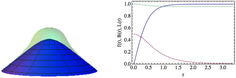
Figure 1 Space-time geometry and profile functions for a subcritical cosmic string of winding number n = 1 with β = 11 . 1, γ = 0 . 19 and ∆ = 0 . 66 π . LEFT: The lower (blue) surface represents the embedding diagram of the spatial metric on the directions transverse to the string, with the string ( r = 0) placed at the top of the figure. The distance between the lower and the upper (green) surfaces represents the magnetic field density on the transverse space. RIGHT: Scalar condensate f ( r ) (solid blue line), magnetic field B ( r ), reescaled from B (0) = 2 . 03 to 1 / 2 at r = 0 to fit nicely in the plot (dashed red), and metric profile function N ( r ) (dotted green).
Figure 1 Space-time geometry and profile functions for a subcritical cosmic string of winding number n = 1 with β = 11 . 1, γ = 0 . 19 and ∆ = 0 . 66 π . LEFT: The lower (blue) surface represents the embedding diagram of the spatial metric on the directions transverse to the string, with the string ( r = 0) placed at the top of the figure. The distance between the lower and the upper (green) surfaces represents the magnetic field density on the transverse space. RIGHT: Scalar condensate f ( r ) (solid blue line), magnetic field B ( r ), reescaled from B (0) = 2 . 03 to 1 / 2 at r = 0 to fit nicely in the plot (dashed red), and metric profile function N ( r ) (dotted green).CC-BY · From the PDF
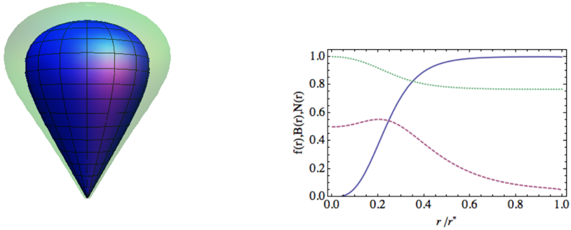
Figure 2 Space-time geometry and profile functions for a supermassive cosmic string of winding n = 3 with β = 11 . 1 and γ = 0 . 19 (∆ = 2 . 84 π ). LEFT: The inner (blue) surface represents the embedding diagram of the spatial metric on the directions transverse to the strings. The cosmic string is at the top of the figure ( r = 0), and the conical singularity at the bottom ( r ∗ = 3 . 9). The distance between the inner and the outer (green) surfaces represents the magnetic field density on the transverse space. RIGHT: Scalar condensate f ( r ) (solid blue line), magnetic field B ( r ) (dashed red), and metric profile function N ( r ) (dotted green). The radial coordinate is measured in units of r ∗ . As in the previous plot the magnetic field is rescaled from B (0) = 2 . 2 to 1 / 2 at r = 0.
Figure 2 Space-time geometry and profile functions for a supermassive cosmic string of winding n = 3 with β = 11 . 1 and γ = 0 . 19 (∆ = 2 . 84 π ). LEFT: The inner (blue) surface represents the embedding diagram of the spatial metric on the directions transverse to the strings. The cosmic string is at the top of the figure ( r = 0), and the conical singularity at the bottom ( r ∗ = 3 . 9). The distance between the inner and the outer (green) surfaces represents the magnetic field density on the transverse space. RIGHT: Scalar condensate f ( r ) (solid blue line), magnetic field B ( r ) (dashed red), and metric profile function N ( r ) (dotted green). The radial coordinate is measured in units of r ∗ . As in the previous plot the magnetic field is rescaled from B (0) = 2 . 2 to 1 / 2 at r = 0.CC-BY · From the PDF
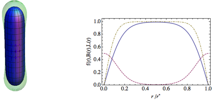
Figure 3 Space-time geometry and profile functions for a configuration (1 , 1) with β = γ = 1, and an inter-string distance is r ∗ = 9 . 4. LEFT: Embedding diagram of the transverse space metric (inner blue surface) and magnetic field density over it (outer green surface). The two strings are located at the top and bottom ends of the figure. RIGHT: Profile functions: scalar field profile function f ( r ) (solid blue line), the magnetic field (dashed red) and L ( r ) (dot-dashed yellow). The radial coordinate is measured in units of r ∗ , and the magnetic field is rescaled from B (0) = 1 to 1 / 2 at r = 0.
Figure 3 Space-time geometry and profile functions for a configuration (1 , 1) with β = γ = 1, and an inter-string distance is r ∗ = 9 . 4. LEFT: Embedding diagram of the transverse space metric (inner blue surface) and magnetic field density over it (outer green surface). The two strings are located at the top and bottom ends of the figure. RIGHT: Profile functions: scalar field profile function f ( r ) (solid blue line), the magnetic field (dashed red) and L ( r ) (dot-dashed yellow). The radial coordinate is measured in units of r ∗ , and the magnetic field is rescaled from B (0) = 1 to 1 / 2 at r = 0.CC-BY · From the PDF
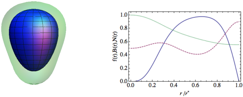
Figure 4 Space-time geometry and profile functions for a configuration (3 , 1) with β = 11 . 1 and γ = 0 . 19. The conical singularity has been resolved by a second cosmic string at r ∗ = 3 . 3. LEFT: Embedding diagram of the transverse space metric (inner blue surface) and magnetic field density over it (outer green surface). The higher and lower winding strings are located at the top and bottom ends of the figure respectively. RIGHT: Profile functions: condensate size f ( r ) (solid blue line), magnetic field (dashed red), and the gravitational potential N ( r ) (dotted green). The radial coordinate is measured in units of r ∗ , and the magnetic field is rescaled from B (0) = 1 . 9 to 1 / 2 at r = 0.
Figure 4 Space-time geometry and profile functions for a configuration (3 , 1) with β = 11 . 1 and γ = 0 . 19. The conical singularity has been resolved by a second cosmic string at r ∗ = 3 . 3. LEFT: Embedding diagram of the transverse space metric (inner blue surface) and magnetic field density over it (outer green surface). The higher and lower winding strings are located at the top and bottom ends of the figure respectively. RIGHT: Profile functions: condensate size f ( r ) (solid blue line), magnetic field (dashed red), and the gravitational potential N ( r ) (dotted green). The radial coordinate is measured in units of r ∗ , and the magnetic field is rescaled from B (0) = 1 . 9 to 1 / 2 at r = 0.CC-BY · From the PDF
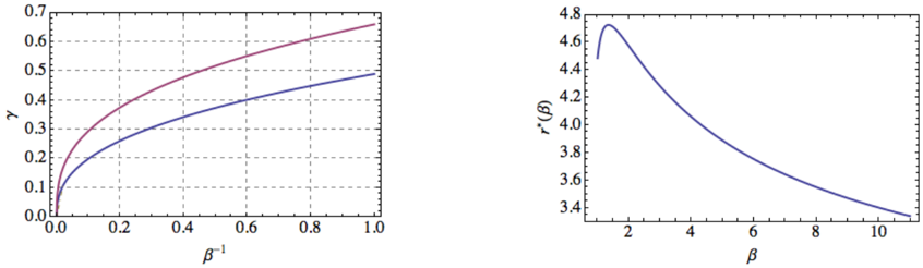
Figure 5 LEFT: The lines represent the possible regular supermassive solutions in the ( γ, 1 /β ) plane for the configurations ( n 1 , n 2 ) = (2 , 1) (bottom) and (3 , 1)( top ). RIGHT: Inter-string distance r ∗ (also related to the size of the transverse space T ) as function of beta on a (3 , 1) configuration. It decays as r ∗ ∼ 5 . 4 β -0 . 2 for β →∞ .
Figure 5 LEFT: The lines represent the possible regular supermassive solutions in the ( γ, 1 /β ) plane for the configurations ( n 1 , n 2 ) = (2 , 1) (bottom) and (3 , 1)( top ). RIGHT: Inter-string distance r ∗ (also related to the size of the transverse space T ) as function of beta on a (3 , 1) configuration. It decays as r ∗ ∼ 5 . 4 β -0 . 2 for β →∞ .CC-BY · From the PDF
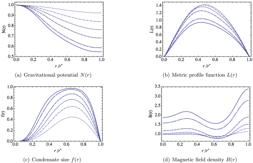
Figure 6 Profile functions of a (3 , 1) configuration for different values of the parameter β . The different line patterns correspond to the same values of beta in all the figures. For example, in the upper left plot the values of β are from bottom to top β = 11 . 1 , 6 . 7 , 2 . 7 , 1 . 7 , 1 . 3, and 1 . 1.
Figure 6 Profile functions of a (3 , 1) configuration for different values of the parameter β . The different line patterns correspond to the same values of beta in all the figures. For example, in the upper left plot the values of β are from bottom to top β = 11 . 1 , 6 . 7 , 2 . 7 , 1 . 7 , 1 . 3, and 1 . 1.CC-BY · From the PDF
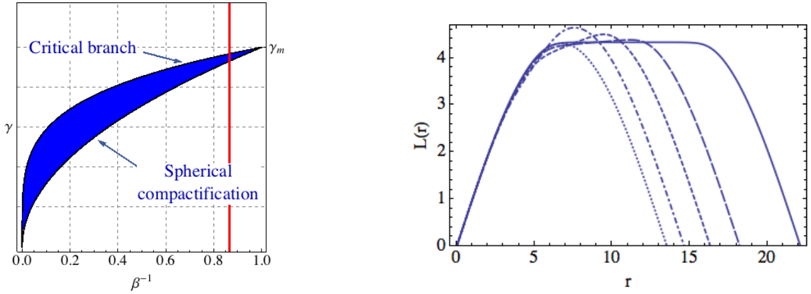
Figure 7 LEFT: Area covered by the different branches of solutions in the large m limit. The limiting curves correspond to the spherical compactification and the ( m/ 2 , m/ 2) solution. The vertical line represents the cut through the parameter space that we do to obtain the curves on the right. In the plot we have denoted by γ m the upper bound for the gravitational coupling (4.6). RIGHT: The form of the internal geometry, L ( r ), in the limit of large flux, m = 50. The dotted line represents the spherical configuration close to the (49 , 1) case. We also plot the (38 , 12), (29 , 21), (26 , 24) and (25 , 25) cases. We see how the solutions interpolate from the perfectly spherical solution to the tubular configuration of 2 critical strings of half the flux separated by a straight segment. The distance between the strings increases substantially as one approaches the even split, the (25 , 25) case. All these curves are computed for β = 1 . 2.
Figure 7 LEFT: Area covered by the different branches of solutions in the large m limit. The limiting curves correspond to the spherical compactification and the ( m/ 2 , m/ 2) solution. The vertical line represents the cut through the parameter space that we do to obtain the curves on the right. In the plot we have denoted by γ m the upper bound for the gravitational coupling (4.6). RIGHT: The form of the internal geometry, L ( r ), in the limit of large flux, m = 50. The dotted line represents the spherical configuration close to the (49 , 1) case. We also plot the (38 , 12), (29 , 21), (26 , 24) and (25 , 25) cases. We see how the solutions interpolate from the perfectly spherical solution to the tubular configuration of 2 critical strings of half the flux separated by a straight segment. The distance between the strings increases substantially as one approaches the even split, the (25 , 25) case. All these curves are computed for β = 1 . 2.CC-BY · From the PDF
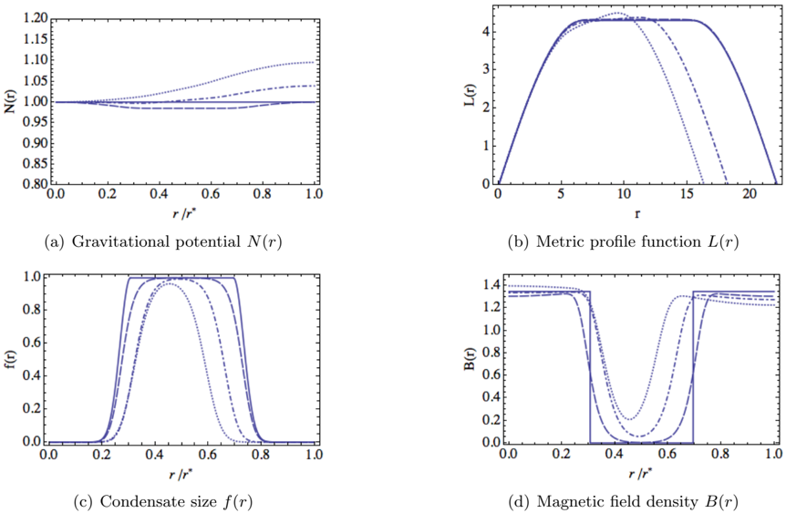
Figure 8 Profile functions of different configurations with a total magnetic flux 2 n = 50 at β = 1 . 818, together with the corresponding large -n approximation (solid line). We show the splittings (25 , 25), (26 , 24) and (29 , 21) with dash-dotted, dashed, and dotted lines respectively.
Figure 8 Profile functions of different configurations with a total magnetic flux 2 n = 50 at β = 1 . 818, together with the corresponding large -n approximation (solid line). We show the splittings (25 , 25), (26 , 24) and (29 , 21) with dash-dotted, dashed, and dotted lines respectively.CC-BY · From the PDF

Verification

Claims the paper makes

The claims and statistics of this paper haven’t been checked yet.

Run the check — free, no account needed. It reads the open-access text and checks the sources it cites.

A few free checks a day · papers already verified open instantly · results are public

Claims other papers make about this one

Each is checked against this paper’s own text: does it say what the citing paper says it does?

Self-check

Percentages, sums and reported differences re-computed from the paper’s own numbers.

The self-check needs the paper’s full text.

Citations

Cites

Research works printed but not linked: 40

  1. 10.1103/PhysRevD.23.852 · DOI
  2. 10.1016/0550-3213(73)90350-7 · DOI
  3. 10.1103/PhysRevD.32.1323 · DOI
  4. 10.1103/PhysRevD.36.3663 · DOI
  5. 10.1103/PhysRevD.40.1011 · DOI
  6. 10.1103/PhysRevD.60.125012 · DOI
  7. B. Meierovich, 2001, Phys. Usp., 44, 981, 10.1070/PU2001v044n10ABEH000935 · DOI
  8. 10.1016/0370-2693(88)90039-1 · DOI
  9. 10.1103/PhysRevD.54.4955 · DOI
  10. 10.1103/PhysRevD.58.103509 · DOI
  11. A. Vilenkin, 1994, Cosmic strings and other topological defects
  12. 10.1103/PhysRevD.43.2521 · DOI
  13. 10.1086/162808 · DOI
  14. B. Linet, 1990, Class. Quant. Grav., 7, L75, 10.1088/0264-9381/7/3/002 · DOI
  15. 10.1016/0550-3213(88)90370-7 · DOI
  16. 10.1016/0550-3213(83)90247-X · DOI · Paper page
  17. 10.1016/0370-2693(84)90589-6 · DOI
  18. 10.1016/j.nuclphysb.2003.12.015 · DOI
  19. Y. Aghababaie ., 2003, J. High Energy Phys., 2003, 037, 10.1088/1126-6708/2003/09/037 · DOI
  20. 10.1007/JHEP02(2013)120 · DOI
  21. 10.1016/0550-3213(90)90248-C · DOI · Paper page
  22. 10.1016/j.nuclphysb.2005.12.020 · DOI
  23. 10.1016/S0370-1573(99)00103-9 · DOI
  24. 10.1103/PhysRevD.31.3288 · DOI
  25. 10.1007/JHEP03(2013)152 · DOI
  26. 10.1103/PhysRev.116.1331 · DOI · Paper page
  27. I. Robinson, 1959, Bull. Acad. Pol. Sci. Ser. Sci. Math. Astron. Phys., 7, 351
  28. H. Nariai, 1950, Sci.Rep. Tohoku Univ., 34, 260
  29. 10.1103/PhysRevD.65.063503 · DOI
  30. 10.1103/PhysRevD.62.085004 · DOI
  31. 10.1103/PhysRevD.51.R6603 · DOI · Paper page
  32. 10.1016/0550-3213(95)00571-4 · DOI · Paper page
  33. 10.1016/0370-2693(96)00210-9 · DOI
  34. G. Dvali, 2004, J. High Energy Phys., 2004, 035, 10.1088/1126-6708/2004/01/035 · DOI · Paper page
  35. 10.1103/PhysRevD.83.085010 · DOI · Paper page
  36. 10.1007/JHEP07(2010)070 · DOI · Paper page
  37. M. Mars, 1993, Class. Quant. Grav., 10, 1865, 10.1088/0264-9381/10/9/026 · DOI
  38. R. Vera, 2002, Classical and Quantum Gravity, 19, 5249, 10.1088/0264-9381/19/20/316 · DOI
  39. 10.1103/PhysRevLett.72.3646 · DOI
  40. 10.1007/978-1-4612-5347-1 · DOI

Cited by

See all 8

Metadata

Authors
Blanco-Pillado, J. J., Reina, B., Sousa, K., & Urrestilla, J.
Venue
Journal of Cosmology and Astroparticle Physics
Published
2014-06-03
Volume
2014
Issue
06
Pages
001-001
ISSN
1475-7516
Cited by
8
References
1

About these checks

Registry, retraction, Cites and statistics results are computed, not judged, with one exception: a printed reference that no index lists is read once by a model before it counts as a citation error. Claims are extracted by a model and kept only when their quote appears verbatim in the text; each cited source is then checked, with a model’s help, for whether it says what the claim relies on. Those verdicts can be wrong — read the claim’s quote and the cited source before relying on one.

Statistics and arithmetic are recomputed, not judged.

Confidence bands are shown only for fields calibrated on our annotated test set. None is calibrated yet, so no band is shown.

What counts as a claim ›How we measure confidence ›How we check this ›

Are you an author, or do you see a problem with this page? Request a review

Data sources

Bibliographic data: Semantic Scholar, OpenAlex, Crossref.

Contains information from the Semantic Scholar Academic Graph Datasets, made available under the ODC Attribution License (ODC-BY 1.0).

Semantic Scholar’s data is described in: Kinney, R., et al. (2023). The Semantic Scholar Open Data Platform. arXiv:2301.10140.