

Simulation-based model selection for dynamical systems in systems and population biology
Open accessThe DOI matches its Crossref record; 43 of the 43 references it cites were found in a registry or an index; 3 of the 9 sources its claims cite were checked for support.
Abstract
Motivation: Computer simulations have become an important tool across the biomedical sciences and beyond. For many important problems several different models or hypotheses exist and choosing which one best describes reality or observed data is not straightforward. We therefore require suitable statistical tools that allow us to choose rationally between different mechanistic models of, e.g. signal transduction or gene regulation networks. This is particularly challenging in systems biology where only a small number of molecular species can be assayed at any given time and all measurements are subject to measurement uncertainty. Results: Here, we develop such a model selection framework based on approximate Bayesian computation and employing sequential Monte Carlo sampling. We show that our approach can be applied across a wide range of biological scenarios, and we illustrate its use on real data describing influenza dynamics and the JAK-STAT signalling pathway. Bayesian model selection strikes a balance between the complexity of the simulation models and their ability to describe observed data. The present approach enables us to employ the whole formal apparatus to any system that can be (efficiently) simulated, even when exact likelihoods are computationally intractable. Contact: ttoni@imperial.ac.uk; m.stumpf@imperial.ac.uk Supplementary information: Supplementary data are available at Bioinformatics online.
Overview
CoChat Summary
TL;DR
The paper develops an approximate Bayesian computation (ABC) model selection framework using sequential Monte Carlo (SMC) for dynamical systems where exact likelihoods are intractable. It demonstrates the method on stochastic reaction kinetics, Gibbs random fields, influenza outbreak data, and JAK-STAT signalling models.
Key findings
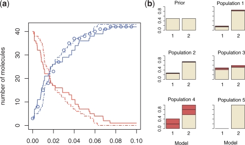
- ABC SMC model selection identified the correct model with high confidence in a synthetic stochastic reaction kinetics example.
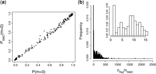
- For Gibbs random fields, ABC SMC estimated posterior model distributions correctly and yielded approximately 50-fold speed-up on average compared with ABC rejection.
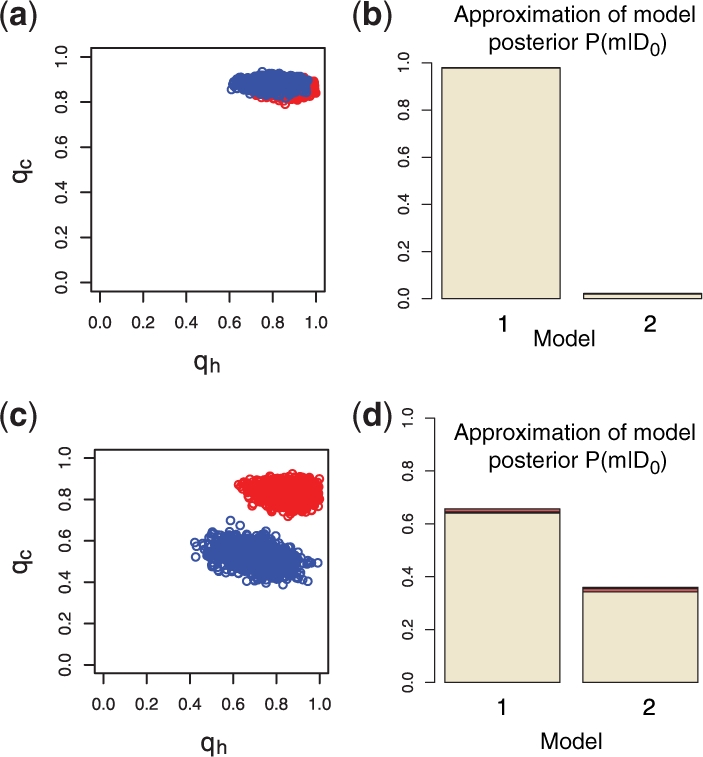
- For influenza outbreaks of the same strain, the posterior probability of the two-parameter shared-parameter model was 0.98 (median over 10 runs), supporting shared epidemiological characteristics.
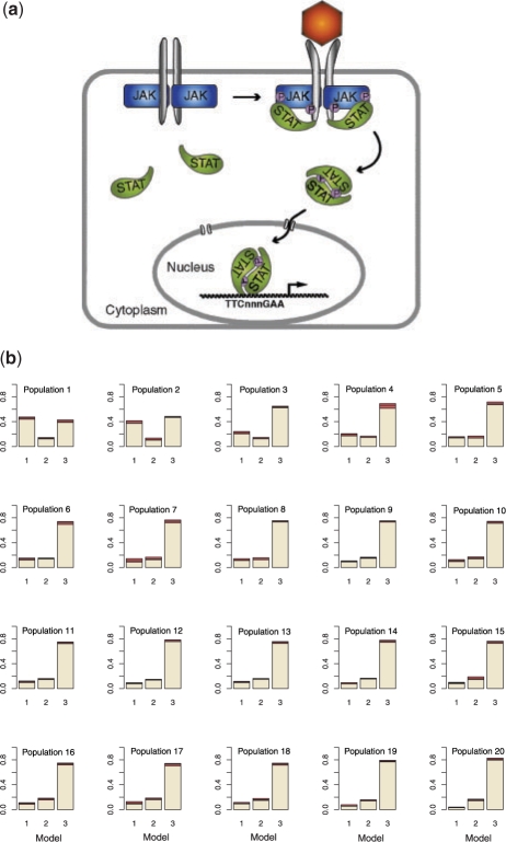
- For JAK-STAT signalling, Bayes factors indicated strong evidence in favour of model 3 over model 1, positive evidence for model 3 over model 2, and positive evidence for model 2 over model 1, favouring the cycling model without a time delay.
Methods
- The authors introduce ABC SMC model selection on the joint space of model indicators and parameters, propagating particles through intermediate distributions with decreasing tolerances.
- The algorithm requires user-defined priors, distance functions, tolerance schedules, and perturbation kernels; in the examples, uniform priors were used for parameters and models.
- Applications included stochastic chemical reaction models, Gibbs random fields with known posteriors, influenza A/B outbreak datasets, and non-nested ordinary and delay differential equation models of STAT5 signalling.
Limitations
- The paper states that routine application to complex models with hundreds or thousands of parameters will require further numerical developments due to the high computational cost of repeated simulations.
- The paper states that SMC-based ABC methods are highly parallelizable and suggests future work exploit this, along with regression adjustment, automatic tolerance schedules, and more sophisticated perturbation kernels.
- Evident from the text: performance depends on choices of distance function, tolerance schedule, and perturbation kernels, and the examples use uniform priors and relatively small particle numbers (e.g. N=500 or N=1000).
Model-written summary. Check it against the paper before relying on it.
Integrity signals
Registry
Cites
Statistics
Figures
Verification
Claims the paper makes
3 Valid · 0 Not valid · 3 Not checked · 28 Own results and interpretations
The cited sources support only part of this claim — read each source’s verdict below.
In the paper
“If ϵ is sufficiently small then this distribution will be a good approximation for the ‘true’ posterior distribution, P(θ|D0).”
§ Simulation-based model selection for dynamical systems in systems and population biology > 1 INTRODUCTION
What the sources say
- Not checked yetcites Beaumont et al., 2002 source
- Partly supportedcites Marjoram et al., 2003 sourceExperimental — accuracy not yet measured
The Abstract paragraph following algorithms C1–C4 supports the ε-limit half of the claim: as ε → ∞ the accepted draws come from the prior, if ε = 0 they come from the posterior density f(θ|𝒟), and 'the choice of ε therefore reflects a tension between computability and accuracy'. However, the paper reserves the label 'approximate Bayesian computation' for the summary-statistic scheme D1–D4, and there it conditions agreement with the true posterior on S being sufficient, noting that 'in practice it will be hard, if not impossible, to identify a suitable set of sufficient statistics'. Its Results make the omission concrete: with S = V the posterior mean of T was ≈1.75 against the 'true' 0.68, and even at ε = 0 with S = (V, H) (Table 4) the mean was 0.59, with the authors sounding 'a note of caution' that summarizing the data can have unexpected effects on the posterior. So the unqualified assertion that a small ε alone makes the ABC output a good approximation to P(θ|D0) is only partly what this source states. (LLM, conf=0.70)
plainstates a cause- Asserted: passes — The authors put it forward as true.
- Checkable: passes — It can be checked against evidence.
- Load-bearing: passes — The paper’s conclusions depend on it.
- Based: passes — The paper gives a reason why it holds.
The cited sources support only part of this claim — read each source’s verdict below.
In the paper
“Both approaches have been applied under the ABC rejection scheme, which is computationally prohibitive for models with even an only moderate number of parameters (Grelaud et al., 2009; Wilkinson, 2007).”
§ Simulation-based model selection for dynamical systems in systems and population biology > 2 ABC FOR MODEL SELECTION
What the sources say
- Partly supportedcites Grelaud et al., 2009 sourceExperimental — accuracy not yet measured
Our copy supports the computational burden of the ABC rejection scheme but not the stated cause: in the 'Exact rejection algorithm' section the authors say the exact (ε=0) version has an 'acceptance probability [that] may be too low to be practical', and in §3.1 (Toy example) 4×10^6 loops yielded as few as 12 acceptances in the worst case; §1.2 adds that the normalising-constant sum 'involves too many terms to be manageable'. However, the paper attributes the difficulty to the dimension of the data/summary statistics and the intractable normalising constant, never to 'even a moderate number of parameters'; it also hedges where the claim states prohibitive as fact, and its overall thrust (§2.1, §4 Discussion) is that ABC is 'naturally tuned' for Gibbs-random-field model choice and implementable on realistic datasets. (LLM, conf=0.70)
- Not checked yetcites Wilkinson, 2007
plainstates a cause- Asserted: passes — The authors put it forward as true.
- Checkable: passes — It can be checked against evidence.
- Load-bearing: passes — The paper’s conclusions depend on it.
- Based: passes — The paper gives a reason why it holds.
- Partly supported
The cited sources support only part of this claim — read each source’s verdict below.
In the paper
“The algorithm presented in Toni et al. (2009) is a special case of the above algorithm for discrete uniform KM kernel and uniform prior distribution of the model P(m).”
§ Simulation-based model selection for dynamical systems in systems and population biology > 2 ABC FOR MODEL SELECTION > 2.1 ABC SMC model selection algorithm on the joint space
What the sources say
- Partly supportedcites Toni et al. (2009) sourceExperimental — accuracy not yet measured
Our copy confirms the structural half of the characterisation: the model-selection scheme treats m ∈ {1,…,M} as an extra discrete parameter and draws m* afresh from the prior π(m) at every population (2.2 Model selection, p. 5, step MS2.1), with uniform perturbation kernels and a discrete uniform model prior in the worked examples (3.1.1, p. 7; Fig. 6 caption 'Population 0 (discrete uniform prior distribution)', 3.3, p. 15). What the source does not support is the subsumption relation itself: Toni et al. nowhere state that their algorithm is a special case of any more general ABC SMC formulation — the only special case they assert is T = 1 reducing ABC SMC to the ABC rejection sampler (2.1, p. 4), and their Appendix B contrasts (rather than nests) their SIS-based scheme with Sisson et al.'s ABC PRC (pp. 21–22). The 'special case of the above algorithm' is therefore the citing authors' own derivation relative to their algorithm, and Toni et al. also present π(m) and K_t generally (uniform or Gaussian), not restricted to the discrete-uniform/uniform-prior setting the claim names. (LLM, conf=0.72)
plain- Asserted: passes — The authors put it forward as true.
- Checkable: passes — It can be checked against evidence.
- Load-bearing: unclear — It is unclear whether the paper’s conclusions depend on it.
- Based: passes — The paper gives a reason why it holds.
- Partly supported
A result the paper reports from its own data — it cites no other source for it, so there is none to check. The quote shows it is in the paper.
In the paper
“This was confirmed by applying our model selection algorithm; the inferred posterior marginal model probability of a two-parameter model was negligible (data not shown).”
§ Simulation-based model selection for dynamical systems in systems and population biology > 3 RESULTS > 3.3 Infuenza infection outbreaks
plain- Asserted: passes — The authors put it forward as true.
- Checkable: passes — It can be checked against evidence.
- Load-bearing: passes — The paper’s conclusions depend on it.
- Based: passes — The paper gives a reason why it holds.
A result the paper reports from its own data — it cites no other source for it, so there is none to check. The quote shows it is in the paper.
In the paper
“Figure 3b shows the marginal posterior distribution of the model; the posterior probability of model 1 is 0.98 (median over 10 runs), which gives unambiguous support to model 1, meaning that outbreaks of the same strain share the same dynamics.”
§ Simulation-based model selection for dynamical systems in systems and population biology > 3 RESULTS > 3.3 Infuenza infection outbreaks
boosted- Asserted: passes — The authors put it forward as true.
- Checkable: passes — It can be checked against evidence.
- Load-bearing: passes — The paper’s conclusions depend on it.
- Based: passes — The paper gives a reason why it holds.
17 more claims
Create a free account to see all 34 claims and to verify the 6 references still open.
- Probably not a substantial claim. 7
- It may state two separate claims as one. 7
Claims other papers make about this one
Each is checked against this paper’s own text: does it say what the citing paper says it does?
The cited source says what the claim attributes to it.
In the citing paper
“In addition to parameter estimation, ABC approaches can also be used for model ranking and selection34.”
From A framework for parameter estimation and model selection from experimental data in systems biology using approximate Bayesian computation (2014) · cites this paper as [34]
Self-check
Percentages, sums and reported differences re-computed from the paper’s own numbers.
Each contradiction between two passages listed here was confirmed by an independent check.
Rated minor: it would not touch a result — a value no result rests on, a p-value that stays on the same side of the significance level, or a conflict that is clerical, resolved elsewhere in the paper, or outside its own findings.
In the paper
§ Simulation-based model selection for dynamical systems in systems and population biology > 3 RESULTS > 3.3 Infuenza infection outbreaks
“find some evidence that model (1) explains the data better than model (1)”
§ Simulation-based model selection for dynamical systems in systems and population biology > 3 RESULTS > 3.3 Infuenza infection outbreaks
“Such a model can be written as (O'Neill et al., 2000) (2)”
Rated minor: it would not touch a result — a value no result rests on, a p-value that stays on the same side of the significance level, or a conflict that is clerical, resolved elsewhere in the paper, or outside its own findings.
In the paper
§ Simulation-based model selection for dynamical systems in systems and population biology > 3 RESULTS > 3.3 Infuenza infection outbreaks
“We thus explore a further model with three parameters, qc1, qc2, qh (model 1), where the two outbreaks share the same within-household characteristics (qh), and compare it against and the four-parameter model (model 2).”
§ Simulation-based model selection for dynamical systems in systems and population biology > 3 RESULTS > 3.3 Infuenza infection outbreaks
“(d) Estimation of a posterior marginal distribution. Model 1 is a two-parameter and model 2 a three-parameter model (1).”
Rated minor: it would not touch a result — a value no result rests on, a p-value that stays on the same side of the significance level, or a conflict that is clerical, resolved elsewhere in the paper, or outside its own findings.
In the paper
§ Simulation-based model selection for dynamical systems in systems and population biology > 3 RESULTS > 3.2 Gibbs random fields
“P(xi+1=xi|xi)=θ1/(1+exp(θ1)) for i=2,…, xn.”
§ Simulation-based model selection for dynamical systems in systems and population biology > 3 RESULTS > 3.2 Gibbs random fields
“Both models, m0 and m1, are defined on a sequence of n binary random variables, x=(x1,…, xn), xi∈{0, 1}”
Rated minor: it would not touch a result — a value no result rests on, a p-value that stays on the same side of the significance level, or a conflict that is clerical, resolved elsewhere in the paper, or outside its own findings.
In the paper
§ Simulation-based model selection for dynamical systems in systems and population biology > 3 RESULTS > 3.2 Gibbs random fields
“m0 is a collection of n i.i.d. Bernoulli random variables with probability θ0/(1+exp(θ0));”
§ Simulation-based model selection for dynamical systems in systems and population biology > 3 RESULTS > 3.2 Gibbs random fields
“θ0 ∼ U(−5, 5)”
Citations
Cites
Model selection and multimodel inference: a practical information-theoretic approach.
Guthery, F. S., Burnham, K. P., & Anderson, D. R. (2003) · The Journal of Wildlife Management · doi:10.2307/3802723 · Cited by 41,495 · cited 2×
“The present approach enables us to employ the whole formal apparatus to any system that can be (efficiently) simulated, even when exact likelihoods are computationally intractable.”
BackgroundMethodGelman, A., Carlin, J. B., Stern, H. S., & Rubin, D. B. (2003) · doi:10.1201/9780429258480 · Cited by 27,276
Kass, R. E., & Raftery, A. E. (1995) · Journal of the American Statistical Association · doi:10.1080/01621459.1995.10476572 · Cited by 12,558
Exact stochastic simulation of coupled chemical reactions
Gillespie, D. T. (1977) · The Journal of Physical Chemistry · doi:10.1021/j100540a008 · Cited by 10,136 · cited 2×
“We simulate synthetic datasets of Y measured at 20 time points using Gillespie algorithm (Gillespie, 1977) from model 2 with parameter k2 =30 and initial conditions X0 =40, Y0”
MethodSequential Monte Carlo Methods in Practice
(2001) · Springer eBooks · doi:10.1007/978-1-4757-3437-9 · Cited by 7,366
Novel Proteinaceous Infectious Particles Cause Scrapie
Prusiner, S. B. (1982) · Science · doi:10.1126/science.6801762 · Cited by 5,118 · cited 3×
“We use data from influenza A (H3N2) outbreaks that occurred in 1977–1978 and 1980–1981 in Tecomseh, Michigan (Addy et al., 1991, Supplementary Table 2), and a second dataset of an influenza B infection outbreak in 1975–1976 and influenza A (H1N1) infection outbreak in 1978–1979 in Seattle, Washington (Longini and Koop…”
BackgroundDarnell, J. E. (1997) · Science · doi:10.1126/science.277.5332.1630 · Cited by 3,979
Approximate Bayesian computation in population genetics
Beaumont, M. A., Zhang, W., & Balding, D. J. (2002) · Genetics · doi:10.1093/genetics/162.4.2025 · Cited by 2,932
Computing Bayes Factors by Combining Simulation and Asymptotic Approximations
Diciccio, T. J., Kass, R. E., Raftery, A., & Wasserman, L. (1997) · Journal of the American Statistical Association · doi:10.1080/01621459.1997.10474045 · Cited by 1,943
Bayesian Data Analysis, 2nd edn
Brix, A. (2005) · Journal of the Royal Statistical Society Series A: Statistics in Society · doi:10.1111/j.1467-985x.2004.00347_4.x · Cited by 1,767
Toni, T., Welch, D., Strelkowa, N., Ipsen, A., & Stumpf, M. P. H. (2009) · Journal of The Royal Society Interface · doi:10.1098/rsif.2008.0172 · Cited by 1,498 · cited 2×
“1b).”
BackgroundSelf-citationUniversally Sloppy Parameter Sensitivities in Systems Biology Models
Gutenkunst, R. N., Waterfall, J. J., Casey, F. P., Brown, K. S., Myers, C. R., & Sethna, J. P. (2007) · PLoS Computational Biology · doi:10.1371/journal.pcbi.0030189 · Cited by 1,261
Sequential Monte Carlo Samplers
Del Moral, P., Doucet, A., & Jasra, A. (2006) · Journal of the Royal Statistical Society Series B: Statistical Methodology · doi:10.1111/j.1467-9868.2006.00553.x · Cited by 1,239
Markov chain Monte Carlo without likelihoods
Marjoram, P., Molitor, J., Plagnol, V., & Tavaré, S. (2003) · Proceedings of the National Academy of Sciences · doi:10.1073/pnas.0306899100 · Cited by 1,199 · cited 1×
“Contact: ttoni@imperial.ac.uk; m.stumpf@imperial.ac.uk Supplementary information: Supplementary data are available at Bioinformatics online.”
BackgroundNedelman, J. R. (2005) · Computational Statistics · doi:10.1007/bf02741321 · Cited by 1,078
Sequential Monte Carlo without likelihoods
Sisson, S. A., Fan, Y., & Tanaka, M. M. (2007) · Proceedings of the National Academy of Sciences · doi:10.1073/pnas.0607208104 · Cited by 856 · cited 1×
“Contact: ttoni@imperial.ac.uk; m.stumpf@imperial.ac.uk Supplementary information: Supplementary data are available at Bioinformatics online.”
BackgroundAn adaptive sequential Monte Carlo method for approximate Bayesian computation
Del Moral, P., Doucet, A., & Jasra, A. (2012) · Statistics and Computing · doi:10.1007/s11222-011-9271-y · Cited by 505
STAT proteins and transcriptional responses to extracellular signals
Horvath, C. M. (2000) · Trends in Biochemical Sciences · doi:10.1016/s0968-0004(00)01624-8 · Cited by 482
Uses and Abuses of Mathematics in Biology
May, R. M. (2004) · Science · doi:10.1126/science.1094442 · Cited by 456 · cited 2×
“Formulating a model to describe, e.g. a signalling pathway or host parasite system, requires us to condense our assumptions and knowledge into a single coherent framework (May, 2004).”
BackgroundNon-linear regression models for Approximate Bayesian Computation
Blum, M. G. B., & François, O. (2010) · Statistics and Computing · doi:10.1007/s11222-009-9116-0 · Cited by 453
Regulation of Interferon-γ-Activated STAT1 by the Ubiquitin-Proteasome Pathway
Kim, T. K., & Maniatis, T. (1996) · Science · doi:10.1126/science.273.5282.1717 · Cited by 401 · cited 1×
“Originally, it had been suggested that STAT5 gets degraded in the nucleus in an ubiquitin-associated way (Kim and Maniatis, 1996), but other evidence suggests that they are dephosphorylated in the nucleus and then trafficked back to the cytoplasm (Köster and Hauser, 1999). d(D0,D ∗)= √∑ t ( y(1)0…”
BackgroundJAK/STAT signalling in Drosophila: insights into conserved regulatory and cellular functions
Arbouzova, N. I., & Zeidler, M. P. (2006) · Development · doi:10.1242/dev.02411 · Cited by 397
Chen, W. W., Schoeberl, B., Jasper, P. J., Niepel, M., Nielsen, U. B., Lauffenburger, D. A., & Sorger, P. K. (2009) · Molecular Systems Biology · doi:10.1038/msb.2008.74 · Cited by 391
Swameye, I., Müller, T. G., Timmer, J., Sandra, O., & Klingmüller, U. (2003) · Proceedings of the National Academy of Sciences · doi:10.1073/pnas.0237333100 · Cited by 316
A Markov random field model for network-based analysis of genomic data
Wei, Z., & Li, H. (2007) · Bioinformatics · doi:10.1093/bioinformatics/btm129 · Cited by 245 · cited 1×
“Both approaches have been applied under theABC rejection scheme, which is computationally prohibitive for models with even an only moderate number of parameters (Grelaud et al., 2009; Wilkinson, 2007).”
MethodKlingmüller, U., Bergelson, S., Hsiao, J. G., & Lodish, H. F. (1996) · Proceedings of the National Academy of Sciences · doi:10.1073/pnas.93.16.8324 · Cited by 189
Prionics or The kinetic basis of prion diseases
Eigen, M. (1996) · Biophysical Chemistry · doi:10.1016/s0301-4622(96)02250-8 · Cited by 187 · cited 3×
“We use data from influenza A (H3N2) outbreaks that occurred in 1977–1978 and 1980–1981 in Tecomseh, Michigan (Addy et al., 1991, Supplementary Table 2), and a second dataset of an influenza B infection outbreak in 1975–1976 and influenza A (H1N1) infection outbreak in 1978–1979 in Seattle, Washington (Longini and Koop…”
BackgroundBayesian ranking of biochemical system models
Vyshemirsky, V., & Girolami, M. A. (2008) · Bioinformatics · doi:10.1093/bioinformatics/btm607 · Cited by 181
Household and Community Transmission Parameters from Final Distributions of Infections in Households
Longini, I. M., & Koopman, J. S. (1982) · Biometrics · doi:10.2307/2530294 · Cited by 174
Model criticism based on likelihood-free inference, with an application to protein network evolution
Ratmann, O., Andrieu, C., Wiuf, C., & Richardson, S. (2009) · Proceedings of the National Academy of Sciences · doi:10.1073/pnas.0807882106 · Cited by 139 · cited 2×
“Contact: ttoni@imperial.ac.uk; m.stumpf@imperial.ac.uk Supplementary information: Supplementary data are available at Bioinformatics online.”
BackgroundMethodAnalyses of Infectious Disease Data from Household Outbreaks by Markov Chain Monte Carlo Methods
O’Neill, P. D., Balding, D. J., Becker, N. G., Eerola, M., & Mollison, D. (2000) · Journal of the Royal Statistical Society Series C (Applied Statistics) · doi:10.1111/1467-9876.00210 · Cited by 138
Spatial Statistics and Computational Methods
Møller, J. (2003) · Lecture notes in statistics · doi:10.1007/978-0-387-21811-3 · Cited by 135
ABC likelihood-free methods for model choice in Gibbs random fields
Grelaud, A., Marin, J.-M., Robert, C. P., Rodolphe, F., & Taly, J.-F. (2009) · Bayesian Analysis · doi:10.1214/09-ba412 · Cited by 119 · cited 3×
“Having convinced ourselves that the novel ABC SMC model selection approach agrees with the analytical model probabilities and those obtained using conventional Bayesian model selection, while outperforming conventional ABC rejection model selection approaches, we can now turn our attention to real…”
MethodInfluentialA Generalized Stochastic Model for the Analysis of Infectious Disease Final Size Data
Addy, C. L., Longini, I. M., & Haber, M. (1991) · Biometrics · doi:10.2307/2532652 · Cited by 117
Ratmann, O., Jørgensen, O., Hinkley, T., Stumpf, M., Richardson, S., & Wiuf, C. (2007) · PLoS Computational Biology · doi:10.1371/journal.pcbi.0030230 · Cited by 98 · cited 2×
“Contact: ttoni@imperial.ac.uk; m.stumpf@imperial.ac.uk Supplementary information: Supplementary data are available at Bioinformatics online.”
BackgroundMethodSelf-citationSBML-PET: a Systems Biology Markup Language-based parameter estimation tool
Zi, Z., & Klipp, E. (2006) · Bioinformatics · doi:10.1093/bioinformatics/btl443 · Cited by 81 · cited 2×
“Instead of x3(t−τ), we propose to model the delay of phosphorylated STAT5 x4 in the nucleus directly and obtain (Zi and Klipp, 2006): ẋ1 = −k1x1EpoRA +2k4x4(t−τ) ẋ4 = k3x3 −k4x4(t−τ).”
Dynamic redistribution of STAT1 protein in IFN signaling visualized by GFP fusion proteins
Köster, M., & Hauser, H. (1999) · European Journal of Biochemistry · doi:10.1046/j.1432-1327.1999.00149.x · Cited by 69 · cited 2×
“…way (Kim and Maniatis, 1996), but other evidence suggests that they are dephosphorylated in the nucleus and then trafficked back to the cytoplasm (Köster and Hauser, 1999). d(D0,D ∗)= √∑ t ( y(1)0 (t)−y∗(1)(t) σ (1) D0 (t) )2 + ( y(2)(t)−y∗(2)(t) σ (2) D0 (t) )2 , with D0 ={y(1)0 ,y (2) 0 }, D∗…”
BackgroundModeling the nonlinear dynamics of cellular signal transduction
TIMMER, J., MÜLLER, T. G., SWAMEYE, I., SANDRA, O., & KLINGMÜLLER, U. (2004) · International Journal of Bifurcation and Chaos · doi:10.1142/s0218127404010461 · Cited by 68 · cited 1×
“The ambiguity of the shutoff mechanism of STAT5 in the nucleus triggered the development of several mathematical models (Müller et al., 2004; Swameye et al., 2003; Timmer and Müller, 2004) describing different hypotheses.”
BackgroundThe ABC of reverse engineering biological signalling systems
Secrier, M., Toni, T., & Stumpf, M. P. H. (2009) · Molecular BioSystems · doi:10.1039/b908951a · Cited by 47
Self-citationTests for cycling in a signalling pathway
Müller, T. G., Faller, D., Timmer, J., Swameye, I., Sandra, O., & Klingmüller, U. (2004) · Journal of the Royal Statistical Society Series C: Applied Statistics · doi:10.1111/j.1467-9876.2004.05148.x · Cited by 33
Parameter Inference for Biochemical Systems that Undergo a Hopf Bifurcation
Kirk, P., Toni, T., & Stumpf, M. P. H. (2008) · Biophysical Journal · doi:10.1529/biophysj.107.126086 · Cited by 31
Self-citationClancy, D., & O’Neill, P. D. (2006) · Scandinavian Journal of Statistics · doi:10.1111/j.1467-9469.2006.00522.x · Cited by 27 · cited 2×
“These data were obtained from two separate outbreaks of the same strain, H3N2, and the question of interest is whether these are characterized by the same epidemiological parameters (this question was previously considered in [21, 22]).”
BackgroundResultBayesian Computation and Model Selection in Population GeneticsPreprint
Excoffier, C. L. D. W. L. (2009) · arXiv (Cornell University) · doi:10.48550/arxiv.0901.2231 · Cited by 17 · cited 1×
“…adjustment techniques that have so far been applied in the parameter estimation ABC framework (Beaumont et al., 2002; Blum and François, 2009; Excoffier, 2009); (ii) from automatic generation of the tolerance schedules (Del Moral et al., 2009); and (iii) by developing more sophisticated…”
Method
Research works printed but not linked: 2
- Jeffreys, 1939, Theory of Probability
- Wilkinson, 2007, Bayesian inference of primate divergence times
Cited by
Approximate Bayesian Computation (ABC) in practice
Csilléry, K., Blum, M. G. B., Gaggiotti, O. E., & François, O. (2010) · Trends in Ecology & Evolution · doi:10.1016/j.tree.2010.04.001 · Cited by 1,302
Approximate Bayesian Computation in Evolution and Ecology
Beaumont, M. A. (2010) · Annual Review of Ecology, Evolution, and Systematics · doi:10.1146/annurev-ecolsys-102209-144621 · Cited by 1,114
Approximate Bayesian computational methods
Marin, J.-M., Pudlo, P., Robert, C. P., & Ryder, R. J. (2012) · Statistics and Computing · doi:10.1007/s11222-011-9288-2 · Cited by 818
“Fearnhead and Prangle (2010) rely on a randomised version of the summary statistics from which they derive a well-calibrated version of ABC, i.e. an algorithm that gives proper predictions of given quantities.”
BackgroundApproximate Bayesian Computation
Sunnåker, M., Busetto, A. G., Numminen, E., Corander, J., Foll, M., & Dessimoz, C. (2013) · PLoS Computational Biology · doi:10.1371/journal.pcbi.1002803 · Cited by 623
“Again, computational improvements for ABC in the space of models have been proposed, such as constructing a particle filter in the joint space of models and parameters [17].”
MethodStatistical inference for stochastic simulation models - theory and application
Hartig, F., Calabrese, J. M., Reineking, B., Wiegand, T., & Huth, A. (2011) · Ecology Letters · doi:10.1111/j.1461-0248.2011.01640.x · Cited by 384
“We have concentrated our discussion mainly on parameter estimation, but once appropriate likelihood approximations are established, model selection and uncertainty estimation can, in principle, be done in the same way as in other statistical applications (e.g. Beaumont 2010; Toni & Stumpf 2010).”
Result
Metadata
- Authors
- Toni, T., & Stumpf, M. P. H.
- Affiliations
- Imperial College London (GB)
- Corresponding author
- Toni, Tina
- Stumpf, Michael P. H.
- Venue
- Bioinformatics
- Publisher
- Oxford University Press (OUP)
- Published
- 2009-10-29
- Volume
- 26
- Issue
- 1
- Pages
- 104-110
- ISSN
- 1367-4803 (ISSN-L)
- 1367-4811
- PMC
- PMC2796821
- OpenAlex
- W2126351705
- Cited by
- 260
- References
- 43
- Citations by year
- 2026: 7 · 2025: 12 · 2024: 11 · 2023: 13 · 2022: 6 · 2021: 19 · 2020: 16 · 2019: 15 · 2018: 19 · 2017: 16 · 2016: 15 · 2015: 20 · 2014: 22 · 2013: 19 · 2012: 18
- FWCI
- 6.70
- Type
- journal article
- Language
- en
- Open access
- hybrid
- doi.org
- Licence
- Locations
- Bioinformatics (publishedVersion, cc-by-nc)
- PubMed Central (publishedVersion, cc-by-nc)
- PubMed (publishedVersion)
- arXiv (Cornell University) (submittedVersion)
- Minerva Access (University of Melbourne) (submittedVersion, cc-by-nc)
- arXiv (Cornell University)
- Funders
- Directorate for Biological Sciences
- Medical Research Council
- Biotechnology and Biological Sciences Research Council (BB/F005210/2, BB/F005210/1, BB/C519670/1, BB/G009374/1)
- Topics
- Life Sciences › Biochemistry, Genetics and Molecular Biology › Molecular Biology › Gene Regulatory Network Analysis
- Physical Sciences › Mathematics › Statistics and Probability › Markov Chains and Monte Carlo Methods
- Social Sciences › Arts and Humanities › History and Philosophy of Science › Philosophy of Biology and Scientific Explanation
- Keywords
- model selection, dynamical systems, approximate Bayesian computation, sequential Monte Carlo, signal transduction, gene regulatory networks, JAK/STAT signaling, population biology, measurement uncertainty, mechanistic model
- MeSH terms
- Algorithms, Animals, Bayes Theorem, Computer Simulation, Data Interpretation, Statistical, Humans, Models, Biological, Population Dynamics, Models, Statistical
About these checks
Registry, retraction, Cites and statistics results are computed, not judged, with one exception: a printed reference that no index lists is read once by a model before it counts as a citation error. Claims are extracted by a model and kept only when their quote appears verbatim in the text; each cited source is then checked, with a model’s help, for whether it says what the claim relies on. Those verdicts can be wrong — read the claim’s quote and the cited source before relying on one.
The claim verdicts this report counts are experimental: their accuracy is not yet measured.
A language model drew the claims from the paper on 2026-10-04, under version 3 of the claim definition (model deepseek-v4.1-flash, prompt extract-v3).
A second model labelled each claim on 2026-10-04 (model jev-1.13-20260917, definition revision gold-guideline-v0.2).
Cited sources are checked with a language model’s help (qwen3.8-omni-flash).
Statistics and arithmetic are recomputed, not judged.
Confidence bands are shown only for fields calibrated on our annotated test set. None is calibrated yet, so no band is shown.
What counts as a claim ›How we measure confidence ›How we check this ›
Are you an author, or do you see a problem with this page? Request a review
Data sources
Bibliographic data: Semantic Scholar, OpenAlex, Crossref.
Contains information from the Semantic Scholar Academic Graph Datasets, made available under the ODC Attribution License (ODC-BY 1.0).
Semantic Scholar’s data is described in: Kinney, R., et al. (2023). The Semantic Scholar Open Data Platform. arXiv:2301.10140.
