

The DOI matches its Crossref record; 23 of the 23 references it cites were found in a registry or an index.
Of maps and grids
Open accessAbstract
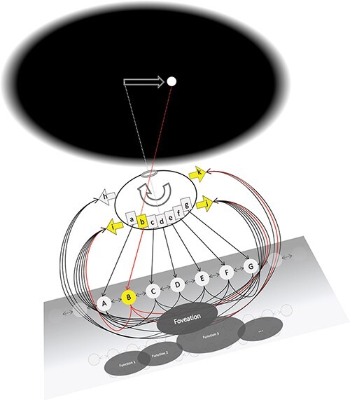
Neuroscience has made remarkable advances in accounting for how the brain performs its various functions. Consciousness, too, is usually approached in functional terms: the goal is to understand how the brain represents information, accesses that information, and acts on it. While useful for prediction, this functional, information-processing approach leaves out the subjective structure of experience: it does not account for how experience feels. Here, we consider a simple model of how a “grid-like” network meant to resemble posterior cortical areas can represent spatial information and act on it to perform a simple “fixation” function. Using standard neuroscience tools, we show how the model represents topographically the retinal position of a stimulus and triggers eye muscles to fixate or follow it. Encoding, decoding, and tuning functions of model units illustrate the working of the model in a way that fully explains what the model does. However, these functional properties have nothing to say about the fact that a human fixating a stimulus would also “see” it—experience it at a location in space. Using the tools of Integrated Information Theory, we then show how the subjective properties of experienced space—its extendedness—can be accounted for in objective, neuroscientific terms by the “cause-effect structure” specified by the grid-like cortical area. By contrast, a “map-like” network without lateral connections, meant to resemble a pretectal circuit, is functionally equivalent to the grid-like system with respect to representation, action, and fixation but cannot account for the phenomenal properties of space.
Overview
The claims and statistics of this paper haven’t been checked yet.
Free: it reads the open-access text and checks the first 5 claims that cite a source we can check. Create a free account to check every claim.
Integrity signals
Registry
Cites
Statistics
Figures



Verification
Claims the paper makes
The claims and statistics of this paper haven’t been checked yet.
Free: it reads the open-access text and checks the first 5 claims that cite a source we can check. Create a free account to check every claim.
Claims other papers make about this one
Each is checked against this paper’s own text: does it say what the citing paper says it does?
The source backs part of the claim, not all of it — or backs it for a different population, condition or comparison.
In the citing paper
“For example, IIT posits that (1) hierarchically organized grid-like cortical structures with lateral and recurrent convergent-divergent connections, such as those found in posterior cortex, are optimally suited for integrating information and thus correspond to the neural substrate of consciousness, 96”
From An integrative, multiscale view on neural theories of consciousness (2024) · cites this paper as [96]
Experimental — accuracy not yet measuredThe source backs part of the claim, not all of it — or backs it for a different population, condition or comparison.
In the citing paper
“For IIT the cause-effect structure of grid-like cortices with recurrent pyramid-like, convergent-divergent connections (such as those found in posterior areas) (Figure 7B) is thought to correspond to a maximum of complexity and thus be sufficient for conscious experience.96,97”
From An integrative, multiscale view on neural theories of consciousness (2024) · cites this paper as [96]
Experimental — accuracy not yet measuredThe cited source says what the claim attributes to it.
In the citing paper
“An important implication of this approach is its rejection of functionalism: two systems may have equivalent (or practically indistinguishable) input-output functions (i.e., respond to identical stimuli in the same way), yet the degree and quality of conscious experience may differ dramatically between systems depending on the cause-effect powers realised by their architectures (Albantakis et al.,”
From Integrated information and predictive processing theories of consciousness: An adversarial collaborative review (2026) · cites this paper as Grasso et al., 2021
The cited source says what the claim attributes to it.
In the citing paper
“For example, an IIT-based analysis of spatial extendedness suggests a grid-like substrate would be required to instantiate this kind of experience, which is consistent with the structure of posterior cortical regions implicated in visual processing (Grasso et al., 2021; Haun & Tononi, 2019).”
From Integrated information and predictive processing theories of consciousness: An adversarial collaborative review (2026) · cites this paper as Grasso et al., 2021
The cited source says what the claim attributes to it.
In the citing paper
“Proponents of IIT have identified the 2D grid-like organisation of posterior cortical networks as a prime candidate for explaining the phenomenal character of spatial extendedness in the visual modality”
From Integrated information and predictive processing theories of consciousness: An adversarial collaborative review (2026) · cites this paper as Grasso et al., 2021
Self-check
Percentages, sums and reported differences re-computed from the paper’s own numbers.
The self-check needs the paper’s full text.
Citations
Cites
Hohwy, J. (2013) · doi:10.1093/acprof:oso/9780199682737.001.0001 · Cited by 1,914
Integrated information theory: from consciousness to its physical substrate
Tononi, G., Boly, M., Massimini, M., & Koch, C. (2016) · Nature Reviews Neuroscience · doi:10.1038/nrn.2016.44 · Cited by 1,727
Self-citationRetinotopic organization in human visual cortex and the spatial precision of functional MRI
Engel, S. (1997) · Cerebral Cortex · doi:10.1093/cercor/7.2.181 · Cited by 1,621
From the phenomenology to the mechanisms of consciousness: integrated information theory 3.0
Oizumi, M., Albantakis, L., & Tononi, G. (2014) · PLoS Computational Biology · doi:10.1371/journal.pcbi.1003588 · Cited by 1,128
Self-citationKriegeskorte, N. (2015) · Annual Review of Vision Science · doi:10.1146/annurev-vision-082114-035447 · Cited by 1,093
Striate cortex of monkey and cat: contrast response function.
Albrecht, D. G., & Hamilton, D. B. (1982) · Journal of Neurophysiology · doi:10.1152/jn.1982.48.1.217 · Cited by 950
Lateral Connectivity and Contextual Interactions in Macaque Primary Visual Cortex
Stettler, D. D., Das, A., Bennett, J., & Gilbert, C. D. (2002) · Neuron · doi:10.1016/s0896-6273(02)01029-2 · Cited by 504
Hlavin, L. (1990) · Neurology · doi:10.1212/wnl.40.2.388-c · Cited by 424
Imaging retinotopic maps in the human brain
Wandell, B. A., & Winawer, J. (2011) · Vision Research · doi:10.1016/j.visres.2010.08.004 · Cited by 373
Martin, J. H. (1989) · Cited by 295
Cited by
An integrative, multiscale view on neural theories of consciousness
Storm, J. F., Klink, P. C., Aru, J., Senn, W., Goebel, R., Pigorini, A., Avanzini, P., Vanduffel, W., Roelfsema, P. R., Massimini, M., et al. (2024) · Neuron · doi:10.1016/j.neuron.2024.02.004 · Cited by 114
“…as those found in posterior cortex, are optimally suited for integrating information and thus correspond to the neural substrate of consciousness, 96 and (2) that phenomenal space—the feeling of extendedness—can be…”
Consciousness and the fallacy of misplaced objectivity
Ellia, F., Hendren, J., Grasso, M., Kozma, C., Mindt, G., P. Lang, J., M. Haun, A., Albantakis, L., Boly, M., & Tononi, G. (2021) · Neuroscience of Consciousness · doi:10.1093/nc/niab032 · Cited by 57
Self-citationVishne, G., Gerber, E. M., Knight, R. T., & Deouell, L. Y. (2023) · Cell Reports · doi:10.1016/j.celrep.2023.112752 · Cited by 46
Dissociating Artificial Intelligence from Artificial Consciousness
Findlay, G., Marshall, W., Albantakis, L., David, I., Mayner, W. G., Koch, C., & Tononi, G. (2024) · arXiv · doi:10.48550/arxiv.2412.04571 · Cited by 41
“…consciousness may split under some concurrent tasks [29], why specific contents of consciousness such as the visual field, temporal flow or mental objects may feel the way they do [40, 41, 91–93], and why consciousness may have evolved due to selective pressure for information integration [94–96].”
Self-citationSpontaneous and Perturbational Complexity in Cortical Cultures
Colombi, I., Nieus, T. R., Massimini, M., & Chiappalone, M. (2021) · Brain Sciences · doi:10.3390/brainsci11111453 · Cited by 29
Metadata
- Authors
- Grasso, M., Haun, A. M., & Tononi, G.
- Affiliations
- University of Wisconsin–Madison (US)
- Corresponding author
- Tononi, Giulio
- Venue
- Neuroscience of Consciousness
- Publisher
- Oxford University Press (OUP)
- Published
- 2021-09-01
- Volume
- 2021
- Issue
- 2
- Pages
- niab022-niab022
- ISSN
- 2057-2107 (ISSN-L)
- PMC
- PMC8452603
- OpenAlex
- W3201266294
- Cited by
- 19
- References
- 23
- Citations by year
- 2026: 5 · 2025: 4 · 2024: 3 · 2023: 2 · 2022: 3 · 2021: 2
- FWCI
- 2.42
- Type
- journal article
- Language
- en
- Open access
- gold
- doi.org
- Licence
- Locations
- Neuroscience of Consciousness (publishedVersion, cc-by)
- Europe PMC (PubMed Central) (publishedVersion, other-oa)
- PubMed Central (publishedVersion, cc-by)
- PubMed (publishedVersion)
- Funders
- Tiny Blue Dot Foundation
- Templeton World Charity Foundation
- Topics
- Social Sciences › Arts and Humanities › Philosophy › Philosophy and Theoretical Science
- Life Sciences › Neuroscience › Cognitive Neuroscience › Neural dynamics and brain function
- Life Sciences › Neuroscience › Cognitive Neuroscience › Visual perception and processing mechanisms
- Keywords
- grid cells, eye fixations, spatial representation, integrated information theory, phenomenal space, subjective experience, causal structure, topographic map
About these checks
Registry, retraction, Cites and statistics results are computed, not judged, with one exception: a printed reference that no index lists is read once by a model before it counts as a citation error. Claims are extracted by a model and kept only when their quote appears verbatim in the text; each cited source is then checked, with a model’s help, for whether it says what the claim relies on. Those verdicts can be wrong — read the claim’s quote and the cited source before relying on one.
Statistics and arithmetic are recomputed, not judged.
Confidence bands are shown only for fields calibrated on our annotated test set. None is calibrated yet, so no band is shown.
What counts as a claim ›How we measure confidence ›How we check this ›
Are you an author, or do you see a problem with this page? Request a review
How to cite
Cite CoChat for the checks on this page, and the paper for its own findings.
- This page
- CoChat. (2026). Citation check: Of maps and grids. https://app.cochat.ai/papers/10.1093/nc/niab022
- The paper
- Grasso, M., Haun, A. M., & Tononi, G. (2021). Of maps and grids. Neuroscience of Consciousness. https://doi.org/10.1093/nc/niab022
Data sources
Bibliographic data: Semantic Scholar, OpenAlex, Crossref.
Contains information from the Semantic Scholar Academic Graph Datasets, made available under the ODC Attribution License (ODC-BY 1.0).
Semantic Scholar’s data is described in: Kinney, R., et al. (2023). The Semantic Scholar Open Data Platform. arXiv:2301.10140.
