CoChat

Model-Based Reinforcement Learning for Ultrasound-Driven Autonomous Microrobots

Open access

Preprint — published as 10.1038/s42256-025-01054-2 · Paper page

The DOI matches its Crossref record; its reference list is not available.

Abstract

AI has catalyzed transformative advancements across multiple sectors, from medical diagnostics to autonomous vehicles, enhancing precision and efficiency. As it ventures into microrobotics, AI offer innovative solutions to the formidable challenge of controlling and manipulating microrobots, which typically operate within imprecise, remotely actuated systems—a task often too complex for human operators. We implement state-of-the-art model-based reinforcement learning for autonomous control of an ultrasound-driven microrobot learning from recurrent imagined environments. Our non-invasive, AI-controlled microrobot offers precise propulsion, which efficiently learns from images in data-scarce environments. Transitioning from a pre-trained simulation environment, we achieve sample-efficient collision avoidance and channel navigation, reaching a 90% success rate in target navigation across various channels within an hour of fine-tuning. Moreover, our model initially successfully generalized in 50% of tasks in new environments, improving to over 90% with 30 minutes of further training. Furthermore, we have showcased real-time manipulation of microrobots within complex vasculatures and across stationary and physiological flows, underscoring AI’s potential to revolutionize microrobotics in biomedical applications, potentially transforming medical procedures.

Overview

The claims and statistics of this paper haven’t been checked yet.

Free: it reads the open-access text and checks the first 5 claims that cite a source we can check. Create a free account to check every claim.

A few free checks a day · papers already verified open instantly · results are public

Integrity signals

Registry

Crossref · 10.1101/2024.09.28.615576

Cites

Statistics

Figures

Fig. 1 An autonomous ultrasound-driven microrobot. a, Left, schematic of the experimental set-up, which has an artificial vascular channel with eight PZTs in an octagonal configuration. Right, the schematic illustrates the behaviour of the microbot under ultrasound activation and details methods for its manipulation. b, Guidelines for manipulating microrobots. c, High-level formulation of the RL problem. The environment is our artificial channel. The RL agent is the microrobot with St actuated by the ultrasound frequency and amplitude to achieve a reward Rt after optimal actions At. d, A world model encoder–decoder structure built to simulate and imagine future states in the environment. e, A simulated game environment designed to pretrain the microrobots, thereby reducing the convergence time during experimental training. f, A recurrent ‘dream’ in the latent space. The microrobot envisions several potential paths towards a target in a dreamed environment, allowing it to dream and train on various possible scenarios simultaneously. g, The microrobot agent executes the optimal action, successfully reaches target 1 and proceeds towards target 2 using a newly imagined path. At, action, Rt, reward; RNN, recurrent neural network; St, state; ƒ𝑛, A𝑛, frequency and amplitude, respectively, of the 𝑛th US wave.
Fig. 1 An autonomous ultrasound-driven microrobot. a, Left, schematic of the experimental set-up, which has an artificial vascular channel with eight PZTs in an octagonal configuration. Right, the schematic illustrates the behaviour of the microbot under ultrasound activation and details methods for its manipulation. b, Guidelines for manipulating microrobots. c, High-level formulation of the RL problem. The environment is our artificial channel. The RL agent is the microrobot with St actuated by the ultrasound frequency and amplitude to achieve a reward Rt after optimal actions At. d, A world model encoder–decoder structure built to simulate and imagine future states in the environment. e, A simulated game environment designed to pretrain the microrobots, thereby reducing the convergence time during experimental training. f, A recurrent ‘dream’ in the latent space. The microrobot envisions several potential paths towards a target in a dreamed environment, allowing it to dream and train on various possible scenarios simultaneously. g, The microrobot agent executes the optimal action, successfully reaches target 1 and proceeds towards target 2 using a newly imagined path. At, action, Rt, reward; RNN, recurrent neural network; St, state; ƒ𝑛, A𝑛, frequency and amplitude, respectively, of the 𝑛th US wave.CC BY · PubMed Central
Fig. 2 Model-based RL structure for an autonomous microrobot. a, The imaging pipeline processes channel images to track microrobot positions. It begins by resizing and cropping the images, followed by segmentation using the segment anything model. Morphological operations and thresholding refine the results. A cluster detection algorithm then identifies relevant clusters, and the CSRT monitors the position of the microbot, providing data on location, area and target information to the world model. b, The world model learns to encode the visual output from the imaging pipeline into a latent representation. It uses an encoder–decoder architecture to reconstruct the images, effectively capturing the latent state (Zt) from the input state (St). The world model simulates future states (St+1, St+2, …) and actions (At, At+1, …) in the latent space, facilitating the prediction of microrobot movements. c, The actor–critic network is iteratively trained within this loop to optimize the policy. It operates in the ‘dreamed’ environment simulated by the world model. This approach reduces the reliance on real-time interactions with the experimental environment. Dec, decoder; Enc, encoder.
Fig. 2 Model-based RL structure for an autonomous microrobot. a, The imaging pipeline processes channel images to track microrobot positions. It begins by resizing and cropping the images, followed by segmentation using the segment anything model. Morphological operations and thresholding refine the results. A cluster detection algorithm then identifies relevant clusters, and the CSRT monitors the position of the microbot, providing data on location, area and target information to the world model. b, The world model learns to encode the visual output from the imaging pipeline into a latent representation. It uses an encoder–decoder architecture to reconstruct the images, effectively capturing the latent state (Zt) from the input state (St). The world model simulates future states (St+1, St+2, …) and actions (At, At+1, …) in the latent space, facilitating the prediction of microrobot movements. c, The actor–critic network is iteratively trained within this loop to optimize the policy. It operates in the ‘dreamed’ environment simulated by the world model. This approach reduces the reliance on real-time interactions with the experimental environment. Dec, decoder; Enc, encoder.CC BY · PubMed Central
Fig. 3 Performance analysis of microrobot navigation in various environments using RL algorithms. a–c, Reward trajectories for a multi-output tributary channel (a), a circuitous channel (b) and a vascular channel (c). Dreamer v.3 (blue) outperformed the hyperparameter-tuned state-of-the-art PPO (green) across simulation steps. Solid lines show smoothed rewards using an exponentially weighted moving average (EWMA; α = 0.002), and shaded areas represent ±1/3 of the standard deviation around the smoothed data. d, Comparison of the PPO and Dreamer algorithms in reaching targets in different channel types: racetrack, tributary (four-out), circuitous, squares, vascular and maze. Box plots show the rate of target achievement evaluated over the final 50 episodes for each trained policy. Boxes represent the interquartile range (IQR; 25th–75th percentiles), the central line indicates the median, whiskers extend to 1.5 × IQR and individual points show outliers. White circles denote the mean. e, Impact of different reward functions on the rate of target achievement. Solid lines represent the centred EWMA of the rate of target achievement (α = 0.1). Shaded regions denote ±1 standard deviation around the EWMA. f, Effects of frame-skipping on performance, presented as a logarithmic plot. Solid lines represent the EWMA of the reward (α = 0.0015), with shaded regions showing ±1/3 of a standard deviation. g, Influence of training ratio on reward dynamics, highlighting consistent performance across various ratios in simulated environments. Solid lines represent the EWMA of the reward (α = 0.008), with shaded regions indicating ±1/3 of a standard deviation. HP, hyperparameter.
Fig. 3 Performance analysis of microrobot navigation in various environments using RL algorithms. a–c, Reward trajectories for a multi-output tributary channel (a), a circuitous channel (b) and a vascular channel (c). Dreamer v.3 (blue) outperformed the hyperparameter-tuned state-of-the-art PPO (green) across simulation steps. Solid lines show smoothed rewards using an exponentially weighted moving average (EWMA; α = 0.002), and shaded areas represent ±1/3 of the standard deviation around the smoothed data. d, Comparison of the PPO and Dreamer algorithms in reaching targets in different channel types: racetrack, tributary (four-out), circuitous, squares, vascular and maze. Box plots show the rate of target achievement evaluated over the final 50 episodes for each trained policy. Boxes represent the interquartile range (IQR; 25th–75th percentiles), the central line indicates the median, whiskers extend to 1.5 × IQR and individual points show outliers. White circles denote the mean. e, Impact of different reward functions on the rate of target achievement. Solid lines represent the centred EWMA of the rate of target achievement (α = 0.1). Shaded regions denote ±1 standard deviation around the EWMA. f, Effects of frame-skipping on performance, presented as a logarithmic plot. Solid lines represent the EWMA of the reward (α = 0.0015), with shaded regions showing ±1/3 of a standard deviation. g, Influence of training ratio on reward dynamics, highlighting consistent performance across various ratios in simulated environments. Solid lines represent the EWMA of the reward (α = 0.008), with shaded regions indicating ±1/3 of a standard deviation. HP, hyperparameter.CC BY · PubMed Central
Fig. 4 Transition of autonomous microrobots from the simulation environment to the physical environment. a, MBRL plot showing the training of microrobots on 32 actions in an experimental racetrack with a square channel. The y axis indicates the reward function, with positive values signalling successful navigation towards the target and negative values indicating crashes. The x axis displays the number of training steps. The solid line shows the EWMA (α = 0.01), and the shaded area represents ±0.5 of the rolling standard deviation (window size of 50) around the EWMA. The reward drops notably at around 300,000 steps due to overfitting to a specific corner of the channel. b, Top, image sequence illustrating the experimental training of microrobots after 100,000 steps. At this early stage, the microrobots frequently failed and reached the target only 20% of the time. Bottom, image sequence showing that after 350,000 training steps, the microrobots demonstrate improved efficiency, reaching the target faster (in seconds) 75% of the time. Red boxes mark the microrobot when it is far from the target, whereas green boxes indicate proximity to the target. The target position is denoted by a circle with a black plus symbol. c, Plot of RL performance illustrating the transition of a pretrained MBRL model from the simulation environment to the physical environment. The score rapidly increased during the simulation phase (blue), dropped after the transition to experiments (marked by a red vertical dashed line) and then increased as the model adapted to the physical environment (green). Solid lines represent the EWMA (α = 0.01) of the reward, with shaded regions indicating ±0.5 of the rolling standard deviation (window size of 50) around the EWMA. d, Micrograph with superimposed images of the navigation steps of microbots within an artificial vasculature. The start and target points are marked by red hollow circles. Arrows in the top left corner indicate all possible movement directions of the microrobots. e–g, Image sequences demonstrating a microrobot navigating an artificial vasculature, starting from the initial position and sequentially reaching three predefined targets: (x1, y1) (e), (x2, y2) (f) and (x3, y3) (g). h, Heat map depicting the relation between speed and position within an artificial vasculature channel. The colour gradient indicates the speed at each position, with darker colours indicating higher speeds and lighter shades denoting slower velocities. Scale bars, 200 µm.
Fig. 4 Transition of autonomous microrobots from the simulation environment to the physical environment. a, MBRL plot showing the training of microrobots on 32 actions in an experimental racetrack with a square channel. The y axis indicates the reward function, with positive values signalling successful navigation towards the target and negative values indicating crashes. The x axis displays the number of training steps. The solid line shows the EWMA (α = 0.01), and the shaded area represents ±0.5 of the rolling standard deviation (window size of 50) around the EWMA. The reward drops notably at around 300,000 steps due to overfitting to a specific corner of the channel. b, Top, image sequence illustrating the experimental training of microrobots after 100,000 steps. At this early stage, the microrobots frequently failed and reached the target only 20% of the time. Bottom, image sequence showing that after 350,000 training steps, the microrobots demonstrate improved efficiency, reaching the target faster (in seconds) 75% of the time. Red boxes mark the microrobot when it is far from the target, whereas green boxes indicate proximity to the target. The target position is denoted by a circle with a black plus symbol. c, Plot of RL performance illustrating the transition of a pretrained MBRL model from the simulation environment to the physical environment. The score rapidly increased during the simulation phase (blue), dropped after the transition to experiments (marked by a red vertical dashed line) and then increased as the model adapted to the physical environment (green). Solid lines represent the EWMA (α = 0.01) of the reward, with shaded regions indicating ±0.5 of the rolling standard deviation (window size of 50) around the EWMA. d, Micrograph with superimposed images of the navigation steps of microbots within an artificial vasculature. The start and target points are marked by red hollow circles. Arrows in the top left corner indicate all possible movement directions of the microrobots. e–g, Image sequences demonstrating a microrobot navigating an artificial vasculature, starting from the initial position and sequentially reaching three predefined targets: (x1, y1) (e), (x2, y2) (f) and (x3, y3) (g). h, Heat map depicting the relation between speed and position within an artificial vasculature channel. The colour gradient indicates the speed at each position, with darker colours indicating higher speeds and lighter shades denoting slower velocities. Scale bars, 200 µm.CC BY · PubMed Central
Fig. 5 Performance of the generalized world model across various environments. a, Reward progression over number of training steps across ten distinct environments, including empty, four squares, racetrack, vascular and several maze configurations. Each coloured line represents the centred EWMA (α = 0.002) of the reward for each environment, with shaded regions indicating ±0.5 of the rolling standard deviation (window size of 1,000 steps). Convergence was faster in simpler environments, whereas more complex ones required extra training steps. After 4.5 million steps, marked by a vertical dashed red line, the model transitioned from pretraining across the ten simulation environments to adaptation within a new multi-output tributary channel. The black curve denotes the average pretraining performance across all environments. Following the transition, the model adapted rapidly, achieving stable performance within ~50,000 steps (approximately 30 min) in the new environment. b, Success rate of targets reached across different environments plotted against number of training steps. The box plots illustrate the variability and distribution of the performance of the MBRL algorithm in successfully reaching targets. Although simpler environments facilitated quicker convergence, our MBRL model consistently attained convergence across all scenarios. Steps are grouped into logarithmic bins from 0 to 4 million steps, and each box summarizes target-reaching rates across a training run within each bin. Boxes indicate the IQR, the horizontal line marks the median, whiskers extend to 1.5 × IQR and outliers are omitted for clarity.
Fig. 5 Performance of the generalized world model across various environments. a, Reward progression over number of training steps across ten distinct environments, including empty, four squares, racetrack, vascular and several maze configurations. Each coloured line represents the centred EWMA (α = 0.002) of the reward for each environment, with shaded regions indicating ±0.5 of the rolling standard deviation (window size of 1,000 steps). Convergence was faster in simpler environments, whereas more complex ones required extra training steps. After 4.5 million steps, marked by a vertical dashed red line, the model transitioned from pretraining across the ten simulation environments to adaptation within a new multi-output tributary channel. The black curve denotes the average pretraining performance across all environments. Following the transition, the model adapted rapidly, achieving stable performance within ~50,000 steps (approximately 30 min) in the new environment. b, Success rate of targets reached across different environments plotted against number of training steps. The box plots illustrate the variability and distribution of the performance of the MBRL algorithm in successfully reaching targets. Although simpler environments facilitated quicker convergence, our MBRL model consistently attained convergence across all scenarios. Steps are grouped into logarithmic bins from 0 to 4 million steps, and each box summarizes target-reaching rates across a training run within each bin. Boxes indicate the IQR, the horizontal line marks the median, whiskers extend to 1.5 × IQR and outliers are omitted for clarity.CC BY · PubMed Central
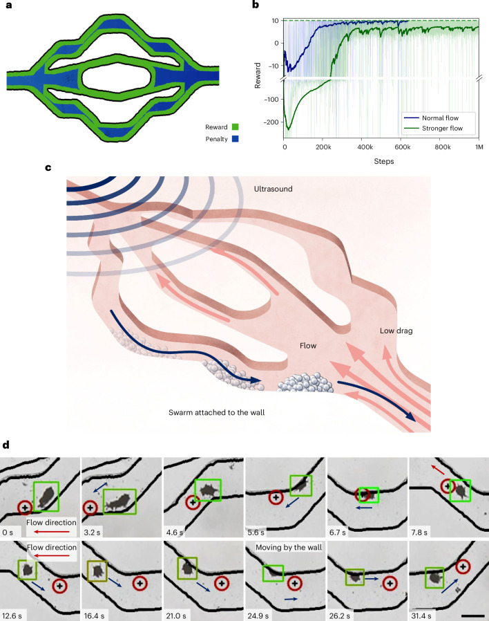
Fig. 6 Autonomous navigation of a microrobot upstream in a flow environment. a, Schematic of the reward function adjusted to promote microrobot navigation close to the wall to minimize drag. b, Graph showing reward progression over time for microrobots in normal (blue line) and stronger (green line) flow conditions, highlighting differences in learning and adaptation. Solid lines represent the EWMAs (α = 0.0015) of the reward. In the normal flow, rewards steadily improve and stabilize around 200,000 steps. In the stronger flow, initial difficulties lead to more negative rewards, but the algorithm shows notable improvement by 400,000 steps. c, Schematic illustrating the behaviour of the microrobot attached to the wall to avoid drag and move against the flow. d, Image sequence showing a microrobot navigating within a microfluidic channel under flow conditions. Initially, when the microrobot was at the centre of the channel (0.0 to 6.7 s), it encountered maximum drag before moving towards the wall (7.8 to 31.4 s), where the drag was minimal. The reduced drag forces at the wall facilitated more stable and controlled navigation. The red arrows indicate the direction of the fluid flow. Scale bar, 200 µm.
Fig. 6 Autonomous navigation of a microrobot upstream in a flow environment. a, Schematic of the reward function adjusted to promote microrobot navigation close to the wall to minimize drag. b, Graph showing reward progression over time for microrobots in normal (blue line) and stronger (green line) flow conditions, highlighting differences in learning and adaptation. Solid lines represent the EWMAs (α = 0.0015) of the reward. In the normal flow, rewards steadily improve and stabilize around 200,000 steps. In the stronger flow, initial difficulties lead to more negative rewards, but the algorithm shows notable improvement by 400,000 steps. c, Schematic illustrating the behaviour of the microrobot attached to the wall to avoid drag and move against the flow. d, Image sequence showing a microrobot navigating within a microfluidic channel under flow conditions. Initially, when the microrobot was at the centre of the channel (0.0 to 6.7 s), it encountered maximum drag before moving towards the wall (7.8 to 31.4 s), where the drag was minimal. The reduced drag forces at the wall facilitated more stable and controlled navigation. The red arrows indicate the direction of the fluid flow. Scale bar, 200 µm.CC BY · PubMed Central
Extended Data Fig. 1 Training with Continuous Actions. a. A plot displaying the relationship between the reward and the steps, illustrating the training progress and performance trends. The solid line represents the exponentially weighted moving average (EWMA) of the reward (α = 0.01), and the shaded region shows ±½ of the rolling standard deviation (window = 50). b. RRT* path planning within an artificial vascular channel. c. A sequence of images showing the microrobot (blue) following the preplanned path (yellow) to reach updated targets (red). The updated targets and intermediate points are marked along the path to visualize the microrobot’s tracking accuracy and performance. Scale bar: 300 µm.
Extended Data Fig. 1 Training with Continuous Actions. a. A plot displaying the relationship between the reward and the steps, illustrating the training progress and performance trends. The solid line represents the exponentially weighted moving average (EWMA) of the reward (α = 0.01), and the shaded region shows ±½ of the rolling standard deviation (window = 50). b. RRT* path planning within an artificial vascular channel. c. A sequence of images showing the microrobot (blue) following the preplanned path (yellow) to reach updated targets (red). The updated targets and intermediate points are marked along the path to visualize the microrobot’s tracking accuracy and performance. Scale bar: 300 µm.CC BY · PubMed Central
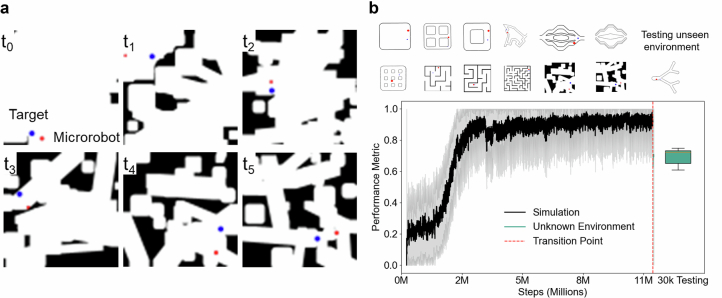
Extended Data Fig. 2 MBRL Model Training and Adaptation. a. Simulated Randomized Environment Complexity: Displays six images, each at a different time step, showing the increasing complexity of simulated randomized environments with obstacles (black) and paths (white). The microrobot (red) navigates towards the target (blue) through these evolving challenges. b. Generalization Across Environments: Depicts adaptation over 12 environments, including 10 original plus 2 newly introduced randomized environments, culminating in a 70% success rate in a novel testing environment, highlighting effective generalization. Solid lines show the exponentially weighted moving average (EWMA, α = 0.01) of success rates, with shaded areas indicating ±½ of the rolling standard deviation (window = 50 steps). A red dashed line marks the environment transition. The final box plot shows the post-adaptation performance, with boxes representing the 25th–75th percentile and whiskers extending to 1.5×IQR.
Extended Data Fig. 2 MBRL Model Training and Adaptation. a. Simulated Randomized Environment Complexity: Displays six images, each at a different time step, showing the increasing complexity of simulated randomized environments with obstacles (black) and paths (white). The microrobot (red) navigates towards the target (blue) through these evolving challenges. b. Generalization Across Environments: Depicts adaptation over 12 environments, including 10 original plus 2 newly introduced randomized environments, culminating in a 70% success rate in a novel testing environment, highlighting effective generalization. Solid lines show the exponentially weighted moving average (EWMA, α = 0.01) of success rates, with shaded areas indicating ±½ of the rolling standard deviation (window = 50 steps). A red dashed line marks the environment transition. The final box plot shows the post-adaptation performance, with boxes representing the 25th–75th percentile and whiskers extending to 1.5×IQR.CC BY · PubMed Central
Extended Data Fig. 3 Microrobot Active and passive Shape-shifting, Demonstrated in Various Configurations. a. Schematic of the experimental setup, showing a straight microchannel equipped with four piezoelectric transducers (PZTs) positioned around an obstacle to manipulate the microrobot. b. Sequence of images illustrating passive microrobot deformation as it navigates through an obstacle using a single PZT activated along the X-axis at 20 volts, demonstrating the robot's ability to passively overcome the barrier. c. Series of images showing active manipulation where two PZTs on the Y-axis are activated, detailing the microrobot's dynamic shape deformation to navigate around the obstacle. d. Image sequence in a bifurcation channel setup where the microrobot encounters an obstacle on one side and actively shape-shifts to maneuver towards the downward path, showcasing advanced control and navigational capabilities. Scale bar: 100 µm.
Extended Data Fig. 3 Microrobot Active and passive Shape-shifting, Demonstrated in Various Configurations. a. Schematic of the experimental setup, showing a straight microchannel equipped with four piezoelectric transducers (PZTs) positioned around an obstacle to manipulate the microrobot. b. Sequence of images illustrating passive microrobot deformation as it navigates through an obstacle using a single PZT activated along the X-axis at 20 volts, demonstrating the robot's ability to passively overcome the barrier. c. Series of images showing active manipulation where two PZTs on the Y-axis are activated, detailing the microrobot's dynamic shape deformation to navigate around the obstacle. d. Image sequence in a bifurcation channel setup where the microrobot encounters an obstacle on one side and actively shape-shifts to maneuver towards the downward path, showcasing advanced control and navigational capabilities. Scale bar: 100 µm.CC BY · PubMed Central
Extended Data Fig. 4 3D Demonstration of Microrobot Manipulation. a. 3D microchannel where microrobots are manipulated. b. Bottom view of the transducer array, illustrating the arrangement of PZTs for 3D control. c. Experimental setup featuring an array of 18 piezoelectric transducers placed in a conical channel, with coupling gel applied between the array and the microchannel for efficient ultrasound transmission. d. Sequence of images showing microrobot movement in 3D as it leaves the focal plane, demonstrating its ability to navigate beyond the primary field of view.
Extended Data Fig. 4 3D Demonstration of Microrobot Manipulation. a. 3D microchannel where microrobots are manipulated. b. Bottom view of the transducer array, illustrating the arrangement of PZTs for 3D control. c. Experimental setup featuring an array of 18 piezoelectric transducers placed in a conical channel, with coupling gel applied between the array and the microchannel for efficient ultrasound transmission. d. Sequence of images showing microrobot movement in 3D as it leaves the focal plane, demonstrating its ability to navigate beyond the primary field of view.CC BY · PubMed Central

Verification

Claims the paper makes

The claims and statistics of this paper haven’t been checked yet.

Free: it reads the open-access text and checks the first 5 claims that cite a source we can check. Create a free account to check every claim.

A few free checks a day · papers already verified open instantly · results are public

Self-check

Percentages, sums and reported differences re-computed from the paper’s own numbers.

The self-check needs the paper’s full text.

Citations

No citation lists for this paper

No citation lists for this paper yet — checked again daily.

References 72 · Cited by 55

Research works printed but not linked: 64

  1. 2020, Deep learning of circulating tumour cells, Nat Mach Intell, 2, 124, 10.1038/s42256-020-0153-x · DOI
  2. 2022, Super-resolution generative adversarial networks of randomly-seeded fields, Nat Mach Intell, 4, 1165, 10.1038/s42256-022-00572-7 · DOI
  3. 2024, β-Variational autoencoders and transformers for reduced-order modelling of fluid flows, Nat Commun, 15, 1361, 10.1038/s41467-024-45578-4 · DOI · Paper page
  4. 10.1038/s41592-020-0792-1 · DOI · Paper page
  5. 2020, Deep Learning in Ultrasound Imaging, Proceedings of the IEEE, 108, 11, 10.1109/JPROC.2019.2932116 · DOI · Paper page
  6. 2023, Deep-learning-enabled brain hemodynamic mapping using resting-state fMRI, npj Digit. Med, 6, 1
  7. 10.1038/s41467-021-26216-9 · DOI · Paper page
  8. 2023, Champion-level drone racing using deep reinforcement learning, Nature, 620, 982, 10.1038/s41586-023-06419-4 · DOI · Paper page
  9. 10.1109/TITS.2021.3054625 · DOI · Paper page
  10. 2020, Machine learning for active matter, Nat Mach Intell, 2, 94, 10.1038/s42256-020-0146-9 · DOI · Paper page
  11. 2024, Machine learning for micro- and nanorobots, Nat Mach Intell, 6, 605, 10.1038/s42256-024-00859-x · DOI
  12. 10.1038/s44222-024-00232-y · DOI
  13. 2024, Medical Microrobots, Annual Review of Biomedical Engineering, 26, 561, 10.1146/annurev-bioeng-081523-033131 · DOI
  14. 10.1146/annurev-bioeng-010510-103409 · DOI · Paper page
  15. 2024, Synchronous and Fully Steerable Active Particle Systems for Enhanced Mimicking of Collective Motion in Nature, Advanced Materials, 36, 2304759, 10.1002/adma.202304759 · DOI
  16. 2020, Micro-rocket robot with all-optic actuating and tracking in blood, Light Sci Appl, 9, 84, 10.1038/s41377-020-0323-y · DOI · Paper page
  17. 2023, Multi-Wavelength Light-Responsive Metal–Phenolic Network-Based Microrobots for Reactive Species Scavenging, Advanced Materials, 35, 2210994, 10.1002/adma.202210994 · DOI
  18. 10.1038/ncomms1550 · DOI · Paper page
  19. 2020, Chemically programmable microrobots weaving a web from hormones, Nat Mach Intell, 2, 711, 10.1038/s42256-020-00248-0 · DOI
  20. 2024, Urease-powered nanobots for radionuclide bladder cancer therapy, Nat. Nanotechnol, 19, 554, 10.1038/s41565-023-01577-y · DOI · Paper page
  21. 10.1126/scirobotics.abd2823 · DOI · Paper page
  22. 2022, Multifunctional 4D-Printed Sperm-Hybrid Microcarriers for Assisted Reproduction, Advanced Materials, 34, 2204257, 10.1002/adma.202204257 · DOI
  23. 10.1063/1.3079655 · DOI · Paper page
  24. 2022, Artificial microtubules for rapid and collective transport of magnetic microcargoes, Nat Mach Intell, 4, 678, 10.1038/s42256-022-00510-7 · DOI
  25. 2022, Magnetic torque–driven living microrobots for increased tumor infiltration, Science Robotics, 7, eabo0665, 10.1126/scirobotics.abo0665 · DOI · Paper page
  26. 10.1021/nl900186w · DOI · Paper page
  27. 2018, Sperm-Hybrid Micromotor for Targeted Drug Delivery, ACS Nano, 12, 327, 10.1021/acsnano.7b06398 · DOI · Paper page
  28. 2024, On-Command Disassembly of Microrobotic Superstructures for Transport and Delivery of Magnetic Micromachines, Advanced Materials, 36, 2310084, 10.1002/adma.202310084 · DOI
  29. 10.1126/sciadv.abb5696 · DOI
  30. 2023, Reconfigurable self-assembly of photocatalytic magnetic microrobots for water purification, Nat Commun, 14, 6969, 10.1038/s41467-023-42674-9 · DOI
  31. 2016, Rotational manipulation of single cells and organisms using acoustic waves, Nat Commun, 7, 11085, 10.1038/ncomms11085 · DOI · Paper page
  32. 2020, Addressable Acoustic Actuation of 3D Printed Soft Robotic Microsystems, Advanced Science, 7, 2001120, 10.1002/advs.202001120 · DOI
  33. 2015, Selectively manipulable acoustic-powered microswimmers, Sci Rep, 5, 9744, 10.1038/srep09744 · DOI · Paper page
  34. 2020, Model-Free Control for Dynamic-Field Acoustic Manipulation Using Reinforcement Learning, IEEE Access, 8, 20597, 10.1109/ACCESS.2020.2969277 · DOI
  35. 10.1126/sciadv.aax3084 · DOI · Paper page
  36. 10.1073/pnas.1920099117 · DOI · Paper page
  37. 10.1038/nature19755 · DOI · Paper page
  38. 1996, Reinforcement Learning: A Survey, Journal of Artificial Intelligence Research, 4, 237, 10.1613/jair.301 · DOI · Paper page
  39. 10.1038/nature14236 · DOI · Paper page
  40. 10.1126/science.aar6404 · DOI · Paper page
  41. 10.1126/scirobotics.abd9285 · DOI · Paper page
  42. 2022, Autonomous environment-adaptive microrobot swarm navigation enabled by deep learning-based real-time distribution planning, Nat Mach Intell, 4, 480, 10.1038/s42256-022-00482-8 · DOI · Paper page
  43. 2024, Autonomous 3D positional control of a magnetic microrobot using reinforcement learning, Nat Mach Intell, 6, 92, 10.1038/s42256-023-00779-2 · DOI
  44. 2022, Smart Magnetic Microrobots Learn to Swim with Deep Reinforcement Learning, Advanced Intelligent Systems, 4, 2200023, 10.1002/aisy.202200023 · DOI
  45. 2024, SonoTransformers: Transformable acoustically activated wireless microscale machines, Proceedings of the National Academy of Sciences, 121, e2314661121, 10.1073/pnas.2314661121 · DOI
  46. 2023, An acoustically controlled helical microrobot, Science Advances, 9, eadh5260, 10.1126/sciadv.adh5260 · DOI
  47. 2024, Robot-assisted chirality-tunable acoustic vortex tweezers for contactless, multifunctional, 4-DOF object manipulation, Science Advances, 10, eadm7698, 10.1126/sciadv.adm7698 · DOI
  48. 10.1021/nn301312z · DOI · Paper page
  49. 2021, Ultrasound-activated ciliary bands for microrobotic systems inspired by starfish, Nat Commun, 12, 6455, 10.1038/s41467-021-26607-y · DOI · Paper page
  50. 10.1109/TASE.2023.3292885 · DOI
  51. 2023, Acoustic Manipulation of Particles in Microfluidic Chips with an Adaptive Controller that Models Acoustic Fields, Advanced Intelligent Systems, 5, 2300058, 10.1002/aisy.202300058 · DOI
  52. Konda, V. & Tsitsiklis, J. Actor-Critic Algorithms. in Advances in Neural Information Processing Systems vol. 12 (MIT Press, 1999).
  53. 10.48550/arXiv.1707.06347 · DOI · Paper page
  54. 1998, Soft Lithography, Angewandte Chemie International Edition, 37, 550, 10.1002/(SICI)1521-3773(19980316)37:5<550::AID-ANIE550>3.0.CO;2-G · DOI · Paper page
  55. 10.48550/arXiv.2304.02643 · DOI · Paper page
  56. Brockman, G. et al. OpenAI Gym. Preprint at http://arxiv.org/abs/1606.01540 (2016). · arXiv
  57. Kalyanakrishnan, S. et al. An Analysis of Frame-skipping in Reinforcement Learning. Preprint at http://arxiv.org/abs/2102.03718 (2021). · arXiv
  58. 10.1126/scirobotics.aba5726 · DOI · Paper page
  59. 2021, Bioinspired acousto-magnetic microswarm robots with upstream motility, Nat Mach Intell, 3, 116, 10.1038/s42256-020-00275-x · DOI · Paper page
  60. 2017, Neutrophil-inspired propulsion in a combined acoustic and magnetic field, Nat Commun, 8, 770, 10.1038/s41467-017-00845-5 · DOI · Paper page
  61. 2022, In vivo acoustic manipulation of microparticles in zebrafish embryos, Science Advances, 8, eabm2785, 10.1126/sciadv.abm2785 · DOI
  62. 2022, Direct sound printing, Nat Commun, 13, 1800, 10.1038/s41467-022-29395-1 · DOI
  63. 2023, Ultrasound trapping and navigation of microrobots in the mouse brain vasculature, Nat Commun, 14, 5889, 10.1038/s41467-023-41557-3 · DOI
  64. 2022, Real-time 3D optoacoustic tracking of cell-sized magnetic microrobots circulating in the mouse brain vasculature, Science Advances, 8, eabm9132, 10.1126/sciadv.abm9132 · DOI · Paper page

Metadata

Authors
Medany, M., Piglia, L., Achenbach, L., Mukkavilli, S. K., & Ahmed, D.
Affiliations
  • ETH Zurich (CH)
  • IBM Research - Zurich (CH)
Corresponding author
Ahmed, Daniel
Venue
Nature Machine Intelligence
Publisher
openRxiv
Published
2024-09-30
Volume
7
Issue
7
Pages
1076-1090
ISSN
2522-5839 (ISSN-L)
OpenAlex
W4411668692
Cited by
55
References
72
Citations by year
2026: 46 · 2025: 8 · 2024: 1
FWCI
16.73
Type
journal article
Language
en
Open access
Locations
  • Nature Machine Intelligence (publishedVersion, cc-by)
  • bioRxiv (Cold Spring Harbor Laboratory) (acceptedVersion, cc-by-nc-nd)
  • Europe PMC (PubMed Central) (publishedVersion, cc-by)
  • PubMed Central (publishedVersion, cc-by)
  • PubMed (publishedVersion)
  • Repository for Publications and Research Data (ETH Zurich) (publishedVersion, cc-by)
  • ETH Zürich Research Collection (cc-by)
Topics
  • Physical Sciences › Physics and Astronomy › Condensed Matter Physics › Micro and Nano Robotics
  • Physical Sciences › Computer Science › Artificial Intelligence › Reinforcement Learning in Robotics
  • Physical Sciences › Engineering › Biomedical Engineering › Soft Robotics and Applications
Keywords
model-based reinforcement learning, sample efficiency, collision avoidance, channel navigation, fine-tuning, generalization across environments, image-based learning

About these checks

Registry, retraction, Cites and statistics results are computed, not judged, with one exception: a printed reference that no index lists is read once by a model before it counts as a citation error. Claims are extracted by a model and kept only when their quote appears verbatim in the text; each cited source is then checked, with a model’s help, for whether it says what the claim relies on. Those verdicts can be wrong — read the claim’s quote and the cited source before relying on one.

Statistics and arithmetic are recomputed, not judged.

Confidence bands are shown only for fields calibrated on our annotated test set. None is calibrated yet, so no band is shown.

What counts as a claim ›How we measure confidence ›How we check this ›

Are you an author, or do you see a problem with this page? Request a review

How to cite

Cite CoChat for the checks on this page, and the paper for its own findings.

This page
CoChat. (2026). Citation check: Model-Based Reinforcement Learning for Ultrasound-Driven Autonomous Microrobots. https://app.cochat.ai/papers/10.1101/2024.09.28.615576
The paper
Medany, M., Piglia, L., Achenbach, L., Mukkavilli, S. K., & Ahmed, D. (2024). Model-Based Reinforcement Learning for Ultrasound-Driven Autonomous Microrobots. Nature Machine Intelligence. https://doi.org/10.1101/2024.09.28.615576

Data sources

Bibliographic data: Semantic Scholar, OpenAlex, Crossref.

Contains information from the Semantic Scholar Academic Graph Datasets, made available under the ODC Attribution License (ODC-BY 1.0).

Semantic Scholar’s data is described in: Kinney, R., et al. (2023). The Semantic Scholar Open Data Platform. arXiv:2301.10140.