Student or educator? Sign up with your school email and get 6 months of Pro free.
CoChat

The DOI matches its Crossref record; 233 of the 241 references it cites were found in a registry or an index.

Explainable Artificial Intelligence for Tabular Data: A Survey

Open access
Sahakyan, Maria, Aung, Zeyar, Rahwan, Talal · 2021 · IEEE Access

Abstract

Machine learning techniques are increasingly gaining attention due to their widespread use in various disciplines across academia and industry. Despite their tremendous success, many such techniques suffer from the “black-box” problem, which refers to situations where the data analyst is unable to explain why such techniques arrive at certain decisions. This problem has fuelled interest in Explainable Artificial Intelligence (XAI), which refers to techniques that can easily be interpreted by humans. Unfortunately, many of these techniques are not suitable for tabular data, which is surprising given the importance and widespread use of tabular data in critical applications such as finance, healthcare, and criminal justice. Also surprising is the fact that, despite the vast literature on XAI, there are still no survey articles to date that focus on tabular data. Consequently, despite the existing survey articles that cover a wide range of XAI techniques, it remains challenging for researchers working on tabular data to go through all of these surveys and extract the techniques that are suitable for their analysis. Our article fills this gap by providing a comprehensive and up-to-date survey of the XAI techniques that are relevant to tabular data. Furthermore, we categorize the references covered in our survey, indicating the type of the model being explained, the approach being used to provide the explanation, and the XAI problem being addressed. Our article is the first to provide researchers with a map that helps them navigate the XAI literature in the context of tabular data.

Overview

The claims and statistics of this paper haven’t been checked yet.

Free: it reads the open-access text and checks the first 5 claims that cite a source we can check. Create a free account to check every claim.

A few free checks a day · papers already verified open instantly · results are public

Integrity signals

Registry

Crossref · 10.1109/access.2021.3116481

Cites

233 of 233 references verified0 citation errors · 0 not checkable

Statistics

Figures

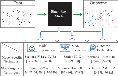
FIGURE 2 An overview of the studies covered in this survey. Explainable AI addresses three problems: (i) Model Explanation , which requires explaining the underlying logic behind a black-box model; (ii) Model inspection , which requires providing visual or textual explanations of certain properties of the underlying model or its outcome, and (iii) Outcome explanation , which requires explaining the model's outcome given an instance of interest, to justify the model's decision. Each of these problems can be addressed with different types of techniques, which can be classified into: (i) model-specific techniques , which are tailored for a particular type of models and cannot readily be generalised to other models, and (ii) model-agnostic techniques , which in principle can be used on any machine learning model. The illustration indicates the sections that cover each problem and each type of techniques, as well as the references covered in each section.
FIGURE 2 An overview of the studies covered in this survey. Explainable AI addresses three problems: (i) Model Explanation , which requires explaining the underlying logic behind a black-box model; (ii) Model inspection , which requires providing visual or textual explanations of certain properties of the underlying model or its outcome, and (iii) Outcome explanation , which requires explaining the model's outcome given an instance of interest, to justify the model's decision. Each of these problems can be addressed with different types of techniques, which can be classified into: (i) model-specific techniques , which are tailored for a particular type of models and cannot readily be generalised to other models, and (ii) model-agnostic techniques , which in principle can be used on any machine learning model. The illustration indicates the sections that cover each problem and each type of techniques, as well as the references covered in each section.CC-BY-NC-ND · From the PDF
Image 2
CC-BY-NC-ND · From the PDF
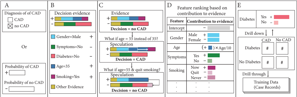
FIGURE 3 An illustration of the ExplainD framework. This illustration describes the intuition behind the ExplainD framework using an example of the diagnosis of obstructive Coronary Artery Disease (CAD). In this example, a physician uses an additive classifier to predict whether a 35-year-old man has CAD. A. The decision of the classifier is that the man has no CAD, because the probability of CAD is smaller than the probability of no CAD. B. An illustration showing how the evidence for not having CAD is stronger than the evidence for having CAD (see how the rectangle marked by '-' is longer than the one marked by '+'). Each evidence consists of multiple additive components corresponding to different features. C. Decision speculation showing how the classification would change if the feature values were different. D. Ranking of the features based on their impact on the classifier's decision. E. To verify whether the classifier's decision match expectations, the user can audit the relationship between the decision label and any given feature. For example, if the feature is 'Diabetes', then the user can slice the training data by label (CAD and No CAD) and feature value (Diabetes and No Diabetes) and examine the data summary in each quadrant to understand how the classifier determined the relationship between Diabetes and CAD.
FIGURE 3 An illustration of the ExplainD framework. This illustration describes the intuition behind the ExplainD framework using an example of the diagnosis of obstructive Coronary Artery Disease (CAD). In this example, a physician uses an additive classifier to predict whether a 35-year-old man has CAD. A. The decision of the classifier is that the man has no CAD, because the probability of CAD is smaller than the probability of no CAD. B. An illustration showing how the evidence for not having CAD is stronger than the evidence for having CAD (see how the rectangle marked by '-' is longer than the one marked by '+'). Each evidence consists of multiple additive components corresponding to different features. C. Decision speculation showing how the classification would change if the feature values were different. D. Ranking of the features based on their impact on the classifier's decision. E. To verify whether the classifier's decision match expectations, the user can audit the relationship between the decision label and any given feature. For example, if the feature is 'Diabetes', then the user can slice the training data by label (CAD and No CAD) and feature value (Diabetes and No Diabetes) and examine the data summary in each quadrant to understand how the classifier determined the relationship between Diabetes and CAD.CC-BY-NC-ND · From the PDF
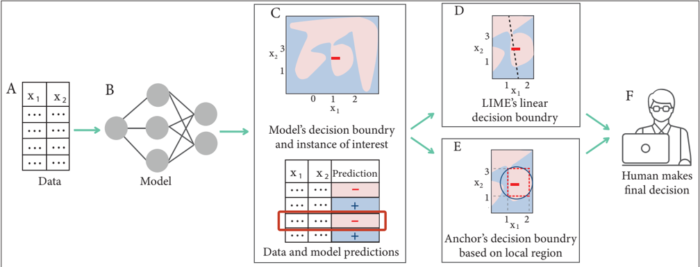
FIGURE 4 An illustration of LIME and Anchors. This illustration describes the intuition behind two alternative techniques, namely LIME and Anchors, on a sample data set with two features. A. The training data set where every example has two features, x 1 and x 2 . B. The data is fed to an ML model such as a neural network. C. The ML model produces a decision boundary, dividing the data space into regions where the data is classified as ' -' (highlighted in pink) and other regions where the data is classified as ' + ' (highlighted in blue). The figure also highlights the instance that requires explanation; see the data point marked as ' -' in the data space. D. The data and the model's predictions are fed to LIME along with the instance that requires explanation. Then, LIME samples instances from the data set and runs a linear model locally, assigning higher weights to the points that are closer to the instance of interest. The outcome of this model is a decision boundary, depicted in the figure as a dashed line, which LIME uses to determine how important each feature is to the classification in this neighbourhood. E. The same as ( D ) but for Anchors instead of LIME. In particular, this technique determines the range of feature values that define an 'anchor', i.e., a region surrounding the given instance where the classification matches the instance; see the dashed rectangle. The output of this technique is the if-then rule defining this region. For example, in our illustration the output would be the following rule: If (1 ≤ x 1 ≤ 2) and (1 ≤ x 2 ≤ 3), then classify the data point as ' -' . F. The analyst is provided with instance-level explanations of how different features influence the model's prediction and makes the final decision accordingly.
FIGURE 4 An illustration of LIME and Anchors. This illustration describes the intuition behind two alternative techniques, namely LIME and Anchors, on a sample data set with two features. A. The training data set where every example has two features, x 1 and x 2 . B. The data is fed to an ML model such as a neural network. C. The ML model produces a decision boundary, dividing the data space into regions where the data is classified as ' -' (highlighted in pink) and other regions where the data is classified as ' + ' (highlighted in blue). The figure also highlights the instance that requires explanation; see the data point marked as ' -' in the data space. D. The data and the model's predictions are fed to LIME along with the instance that requires explanation. Then, LIME samples instances from the data set and runs a linear model locally, assigning higher weights to the points that are closer to the instance of interest. The outcome of this model is a decision boundary, depicted in the figure as a dashed line, which LIME uses to determine how important each feature is to the classification in this neighbourhood. E. The same as ( D ) but for Anchors instead of LIME. In particular, this technique determines the range of feature values that define an 'anchor', i.e., a region surrounding the given instance where the classification matches the instance; see the dashed rectangle. The output of this technique is the if-then rule defining this region. For example, in our illustration the output would be the following rule: If (1 ≤ x 1 ≤ 2) and (1 ≤ x 2 ≤ 3), then classify the data point as ' -' . F. The analyst is provided with instance-level explanations of how different features influence the model's prediction and makes the final decision accordingly.CC-BY-NC-ND · From the PDF
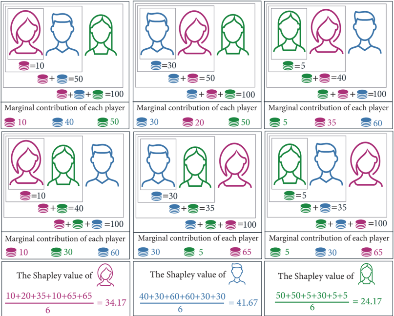
FIGURE 5 An illustration of the Shapley Value. In a coalitional game, every subset of players is called a 'coalition', and the game specifies a value for every coalition indicating the quality of its outcome. The Shapley value is a formula introduced by Lloyd Shapley [58] to fairly measure the contribution of each player to the coalition consisting of all players. This is done by considering all possible joining orders of the players. Given the three players in our example, namely Red, Blue and Green, one possible joining order is that Red joined first, followed by Blue, then Green (see the top-left corner). Another possible joining order is that Green joined first, followed by Red, then Blue (top-right corner). For every joining order, the Shapley value computes the 'marginal contribution' of each player, which is the difference in value caused when that player joins the coalition. For example, given the joining order in the top-left corner, the marginal contribution of Red, Blue and Green is 10, 40, and 50, respectively. Then, the Shapley value of each player is defined as its average marginal contribution, taken over all joining orders (see the bottom row of the figure).
FIGURE 5 An illustration of the Shapley Value. In a coalitional game, every subset of players is called a 'coalition', and the game specifies a value for every coalition indicating the quality of its outcome. The Shapley value is a formula introduced by Lloyd Shapley [58] to fairly measure the contribution of each player to the coalition consisting of all players. This is done by considering all possible joining orders of the players. Given the three players in our example, namely Red, Blue and Green, one possible joining order is that Red joined first, followed by Blue, then Green (see the top-left corner). Another possible joining order is that Green joined first, followed by Red, then Blue (top-right corner). For every joining order, the Shapley value computes the 'marginal contribution' of each player, which is the difference in value caused when that player joins the coalition. For example, given the joining order in the top-left corner, the marginal contribution of Red, Blue and Green is 10, 40, and 50, respectively. Then, the Shapley value of each player is defined as its average marginal contribution, taken over all joining orders (see the bottom row of the figure).CC-BY-NC-ND · From the PDF
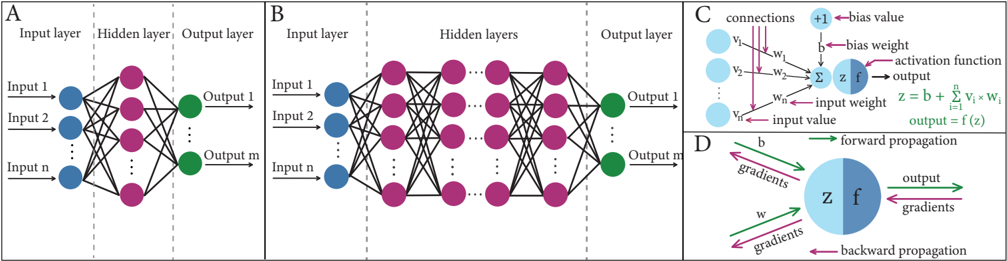
FIGURE 6 An illustration of neural networks and backward propagation. The nodes represent neurons, which belong to either the input layer, the output layer, or any of the hidden layers in between. A. An illustration of Artificial Neural Network (ANN). B. An illustration of Deep Neural Network (DNN), where the number of hidden layers is much larger than in a typical ANN. C. An illustration of the inner workings of neurons in hidden layers. D. Forward propagation refers to the typical flow within an ANN or DNN, which starts from the input layer, goes through the hidden layers, and ends at the output layer. In backward propagation, for each output node, the derivative of the prediction error is calculated with respect to the weights of the edges pointing to that node. The results are then used to perform similar calculations but for the layer before the last, and then for the layer before it, etc., all the way back to the first layer. Finally, the gradient values are subtracted from the weights to minimize the error.
FIGURE 6 An illustration of neural networks and backward propagation. The nodes represent neurons, which belong to either the input layer, the output layer, or any of the hidden layers in between. A. An illustration of Artificial Neural Network (ANN). B. An illustration of Deep Neural Network (DNN), where the number of hidden layers is much larger than in a typical ANN. C. An illustration of the inner workings of neurons in hidden layers. D. Forward propagation refers to the typical flow within an ANN or DNN, which starts from the input layer, goes through the hidden layers, and ends at the output layer. In backward propagation, for each output node, the derivative of the prediction error is calculated with respect to the weights of the edges pointing to that node. The results are then used to perform similar calculations but for the layer before the last, and then for the layer before it, etc., all the way back to the first layer. Finally, the gradient values are subtracted from the weights to minimize the error.CC-BY-NC-ND · From the PDF
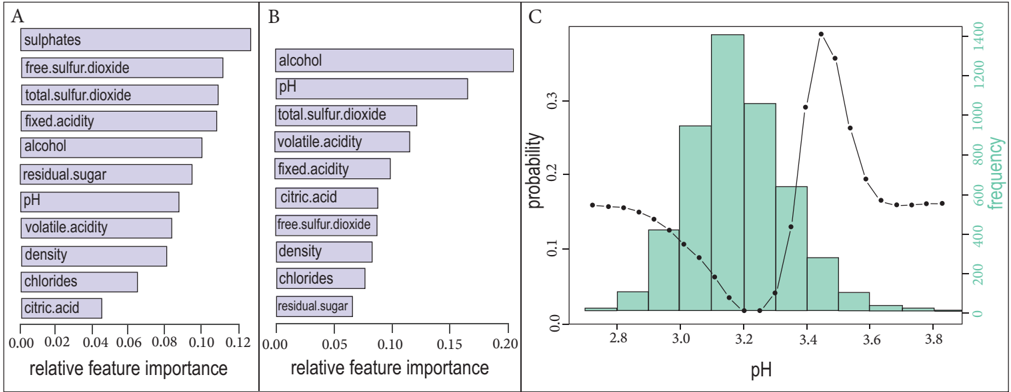
FIGURE 7 An illustration of feature importance and the VEC curve. This example uses a data set on white wine quality [101], consisting of 11 features and an output variable representing the quality of wine on a scale from 3 to 9. A. Bar plot representing feature importance based on the regression analysis of the white wine quality data set, where the goal is to predict human expert taste preferences. B. Bar plot representing the two-dimensional interactions between 'sulphates' (since it has the highest importance in Fig. 7A) and each of the remaining features. This reveals that, when predicting wine quality, alcohol and pH have higher interactions with sulphate compared to the other features. C. Analysis of the white wine quality data set to classify wine as either low quality (where the output variable is < 6) or high quality (where the output variable is ≥ 6). In addition to the histogram of pH (which is the most indicative feature of wine quality according to the paper), the figure shows the Variable Effect Characteristic (VEC) curve, which represents the influence of pH on the model's classification. A non-linear influence of the pH can be observed, highlighting the fact the pH values within the range [3 . 4 , 3 . 5] maximizes the probability of wine quality being classified as high.
FIGURE 7 An illustration of feature importance and the VEC curve. This example uses a data set on white wine quality [101], consisting of 11 features and an output variable representing the quality of wine on a scale from 3 to 9. A. Bar plot representing feature importance based on the regression analysis of the white wine quality data set, where the goal is to predict human expert taste preferences. B. Bar plot representing the two-dimensional interactions between 'sulphates' (since it has the highest importance in Fig. 7A) and each of the remaining features. This reveals that, when predicting wine quality, alcohol and pH have higher interactions with sulphate compared to the other features. C. Analysis of the white wine quality data set to classify wine as either low quality (where the output variable is < 6) or high quality (where the output variable is ≥ 6). In addition to the histogram of pH (which is the most indicative feature of wine quality according to the paper), the figure shows the Variable Effect Characteristic (VEC) curve, which represents the influence of pH on the model's classification. A non-linear influence of the pH can be observed, highlighting the fact the pH values within the range [3 . 4 , 3 . 5] maximizes the probability of wine quality being classified as high.CC-BY-NC-ND · From the PDF
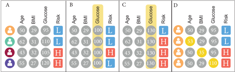
FIGURE 8 An illustration describing how Partial Dependence Plots (PDPs) are computed. This example is based on a data set predicting the risk of developing diabetes, where each row represents a patient, and each column represents a feature. The 'Risk' column is the output of the predictive model (H means High risk, while L means How risk). A. The original feature values of each patient. B. If the analyst wants to examine the impact of glucose on the prediction, partial dependence can be applied by varying the value of glucose while keeping all other features intact, to determine how glucose affects the prediction. In this example, the glucose value is set to 100 for all patients, which changes the prediction of one patient from high risk to low risk. C. The glucose value is now set to 130 for all patients, which changes the prediction of one patient from low risk to high risk. The findings in Fig. 8B and 8C suggest that there is partial dependence between glucose and the prediction. D. Prospector-one of many PDP-based techniques-can also be used for local inspection. In this illustration, all rows represent the same patient. The first row corresponds to the original feature values of that patient, while each of the remaining rows corresponds to a change in one of those values, which is highlighted in yellow. As can be seen, changing the age does not change the prediction, while changing BMI or glucose changes the prediction from low risk to high risk.
FIGURE 8 An illustration describing how Partial Dependence Plots (PDPs) are computed. This example is based on a data set predicting the risk of developing diabetes, where each row represents a patient, and each column represents a feature. The 'Risk' column is the output of the predictive model (H means High risk, while L means How risk). A. The original feature values of each patient. B. If the analyst wants to examine the impact of glucose on the prediction, partial dependence can be applied by varying the value of glucose while keeping all other features intact, to determine how glucose affects the prediction. In this example, the glucose value is set to 100 for all patients, which changes the prediction of one patient from high risk to low risk. C. The glucose value is now set to 130 for all patients, which changes the prediction of one patient from low risk to high risk. The findings in Fig. 8B and 8C suggest that there is partial dependence between glucose and the prediction. D. Prospector-one of many PDP-based techniques-can also be used for local inspection. In this illustration, all rows represent the same patient. The first row corresponds to the original feature values of that patient, while each of the remaining rows corresponds to a change in one of those values, which is highlighted in yellow. As can be seen, changing the age does not change the prediction, while changing BMI or glucose changes the prediction from low risk to high risk.CC-BY-NC-ND · From the PDF
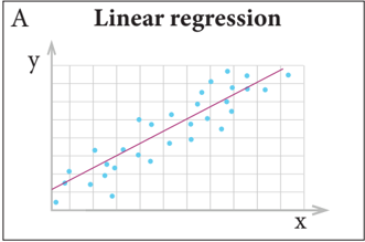
FIGURE 9 An illustration of some popular types of interpretable models.
FIGURE 9 An illustration of some popular types of interpretable models.CC-BY-NC-ND · From the PDF
Image 10
CC-BY-NC-ND · From the PDF
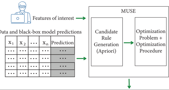
FIGURE 10 An illustration of the algorithmic flow of the MUSE approach. MUSE (which stands for Model Understanding through Subspace Explanations) takes as input the data along with the predictions of a black-box model, as well as the features of interest that are specified by the user. Then, MUSE generates decision rules based on the features of interest. For each such rule, it uses an objective function that jointly optimizes for fidelity to the original model, unambiguity and interpretability of the explanations. Finally, it gives the output in the form of customized explanations.
FIGURE 10 An illustration of the algorithmic flow of the MUSE approach. MUSE (which stands for Model Understanding through Subspace Explanations) takes as input the data along with the predictions of a black-box model, as well as the features of interest that are specified by the user. Then, MUSE generates decision rules based on the features of interest. For each such rule, it uses an objective function that jointly optimizes for fidelity to the original model, unambiguity and interpretability of the explanations. Finally, it gives the output in the form of customized explanations.CC-BY-NC-ND · From the PDF
Image 12
CC-BY-NC-ND · From the PDF
Image 13
CC-BY-NC-ND · From the PDF
Image 14
CC-BY-NC-ND · From the PDF

Verification

Claims the paper makes

The claims and statistics of this paper haven’t been checked yet.

Free: it reads the open-access text and checks the first 5 claims that cite a source we can check. Create a free account to check every claim.

A few free checks a day · papers already verified open instantly · results are public

Self-check

Percentages, sums and reported differences re-computed from the paper’s own numbers.

The self-check needs the paper’s full text.

Citations

Cites

Show all 241 references

Research works printed but not linked: 10

  1. wang, 2017, A Bayesian framework for learning rule sets for interpretable classification, J Mach Learn Res, 18, 2357
  2. molnar, 2021, Interpretable Machine Learning A Guide for Making Black Box Models Explainable
  3. molnar, 2019, Interpretable Machine Learning A Guide for Making Black Box Models Explainable
  4. saabas, 2019, Treeinterpreter Python Package
  5. 2021, The impact of the General Data Protection Regulation (GDPR) on Artificial Intelligence
  6. 2021, Providing Explainable AI Through Advanced Knowledge Graphs
  7. 2021, Model Interpretability in Azure Machine Learning
  8. 2021, Explainable Machine Learning Challenge
  9. chipman, 1998, Making sense of a forest of trees, Proc 30th Symp Interface, 29, 84
  10. angwin, 2016, Machine bias There’s software used across the country to predict future criminals And it’s biased against blacks

Cited by

See all 136

Metadata

Authors
Sahakyan, M., Aung, Z., & Rahwan, T.
Affiliations
  • New York University Abu Dhabi (AE)
  • Khalifa University of Science and Technology (AE)
Venue
IEEE Access
Published
2021
Volume
9
Pages
135392-135422
ISSN
2169-3536 (ISSN-L)
OpenAlex
W3201854521
Cited by
135
References
241
Citations by year
2026: 17 · 2025: 37 · 2024: 43 · 2023: 20 · 2022: 18
FWCI
7.16
Type
journal article
Language
en
Open access
Locations
  • IEEE Access (publishedVersion, cc-by-nc-nd)
  • DOAJ (DOAJ: Directory of Open Access Journals) (submittedVersion, cc-by-sa)
Funders
Khalifa University, Abu Dhabi, UAE, by providing a Ph.D. Scholarship and Research Facilities
Topics
  • Physical Sciences › Computer Science › Artificial Intelligence › Explainable Artificial Intelligence (XAI)
  • Physical Sciences › Computer Science › Artificial Intelligence › Privacy-Preserving Technologies in Data
  • Physical Sciences › Computer Science › Artificial Intelligence › Machine Learning and Data Classification
Keywords
explainable AI, tabular data, black box problem, model interpretability, explanation methods, model types

About these checks

Registry, retraction, Cites and statistics results are computed, not judged, with one exception: a printed reference that no index lists is read once by a model before it counts as a citation error. Claims are extracted by a model and kept only when their quote appears verbatim in the text; each cited source is then checked, with a model’s help, for whether it says what the claim relies on. Those verdicts can be wrong — read the claim’s quote and the cited source before relying on one.

Statistics and arithmetic are recomputed, not judged.

Confidence bands are shown only for fields calibrated on our annotated test set. None is calibrated yet, so no band is shown.

What counts as a claim ›How we measure confidence ›How we check this ›

Are you an author, or do you see a problem with this page? Request a review

How to cite

Cite CoChat for the checks on this page, and the paper for its own findings.

This page
CoChat. (2026). Citation check: Explainable Artificial Intelligence for Tabular Data: A Survey. https://app.cochat.ai/papers/10.1109/access.2021.3116481
The paper
Sahakyan, M., Aung, Z., & Rahwan, T. (2021). Explainable Artificial Intelligence for Tabular Data: A Survey. IEEE Access. https://doi.org/10.1109/access.2021.3116481

Data sources

Bibliographic data: Semantic Scholar, OpenAlex, Crossref.

Contains information from the Semantic Scholar Academic Graph Datasets, made available under the ODC Attribution License (ODC-BY 1.0).

Semantic Scholar’s data is described in: Kinney, R., et al. (2023). The Semantic Scholar Open Data Platform. arXiv:2301.10140.