

The DOI matches its Crossref record; 47 of the 47 references it cites were found in a registry or an index.
A Graph-Transformer for Whole Slide Image Classification
Open accessPublished version of a preprint
Abstract
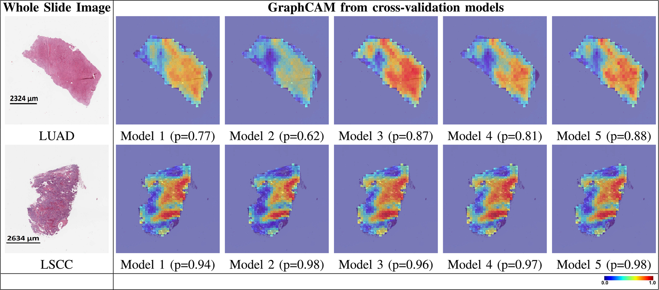
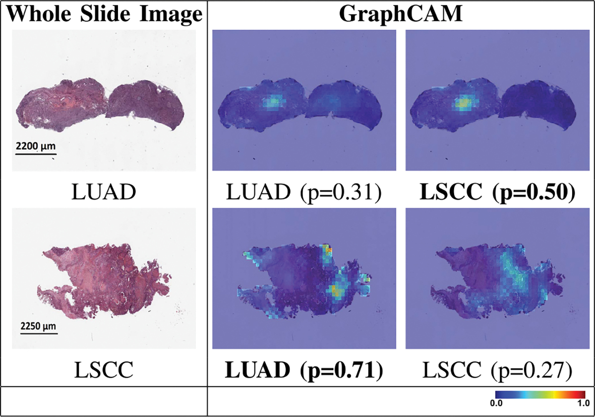
Deep learning is a powerful tool for whole slide image (WSI) analysis. Typically, when performing supervised deep learning, a WSI is divided into small patches, trained and the outcomes are aggregated to estimate disease grade. However, patch-based methods introduce label noise during training by assuming that each patch is independent with the same label as the WSI and neglect overall WSI-level information that is significant in disease grading. Here we present a Graph-Transformer (GT) that fuses a graph-based representation of an WSI and a vision transformer for processing pathology images, called GTP, to predict disease grade. We selected 4,818 WSIs from the Clinical Proteomic Tumor Analysis Consortium (CPTAC), the National Lung Screening Trial (NLST), and The Cancer Genome Atlas (TCGA), and used GTP to distinguish adenocarcinoma (LUAD) and squamous cell carcinoma (LSCC) from adjacent non-cancerous tissue (normal). First, using NLST data, we developed a contrastive learning framework to generate a feature extractor. This allowed us to compute feature vectors of individual WSI patches, which were used to represent the nodes of the graph followed by construction of the GTP framework. Our model trained on the CPTAC data achieved consistently high performance on three-label classification (normal versus LUAD versus LSCC: mean accuracy = 91.2 ± 2.5%) based on five-fold cross-validation, and mean accuracy = 82.3 ± 1.0% on external test data (TCGA). We also introduced a graph-based saliency mapping technique, called GraphCAM, that can identify regions that are highly associated with the class label. Our findings demonstrate GTP as an interpretable and effective deep learning framework for WSI-level classification.
Overview
The claims and statistics of this paper haven’t been checked yet.
Run the check — free, no account needed. It reads the open-access text and checks the sources it cites.
Integrity signals
Registry
Cites
Statistics
Figures
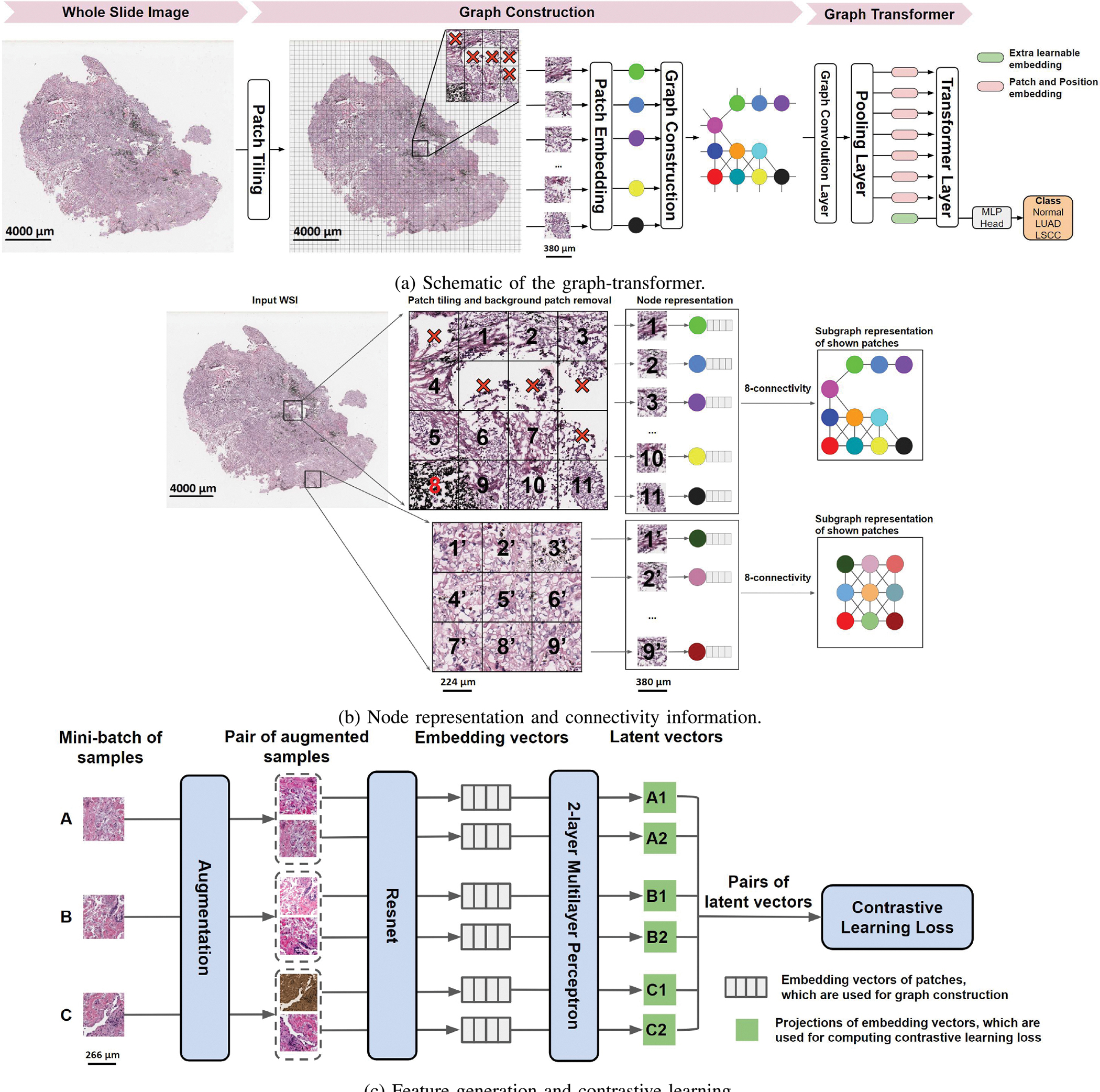
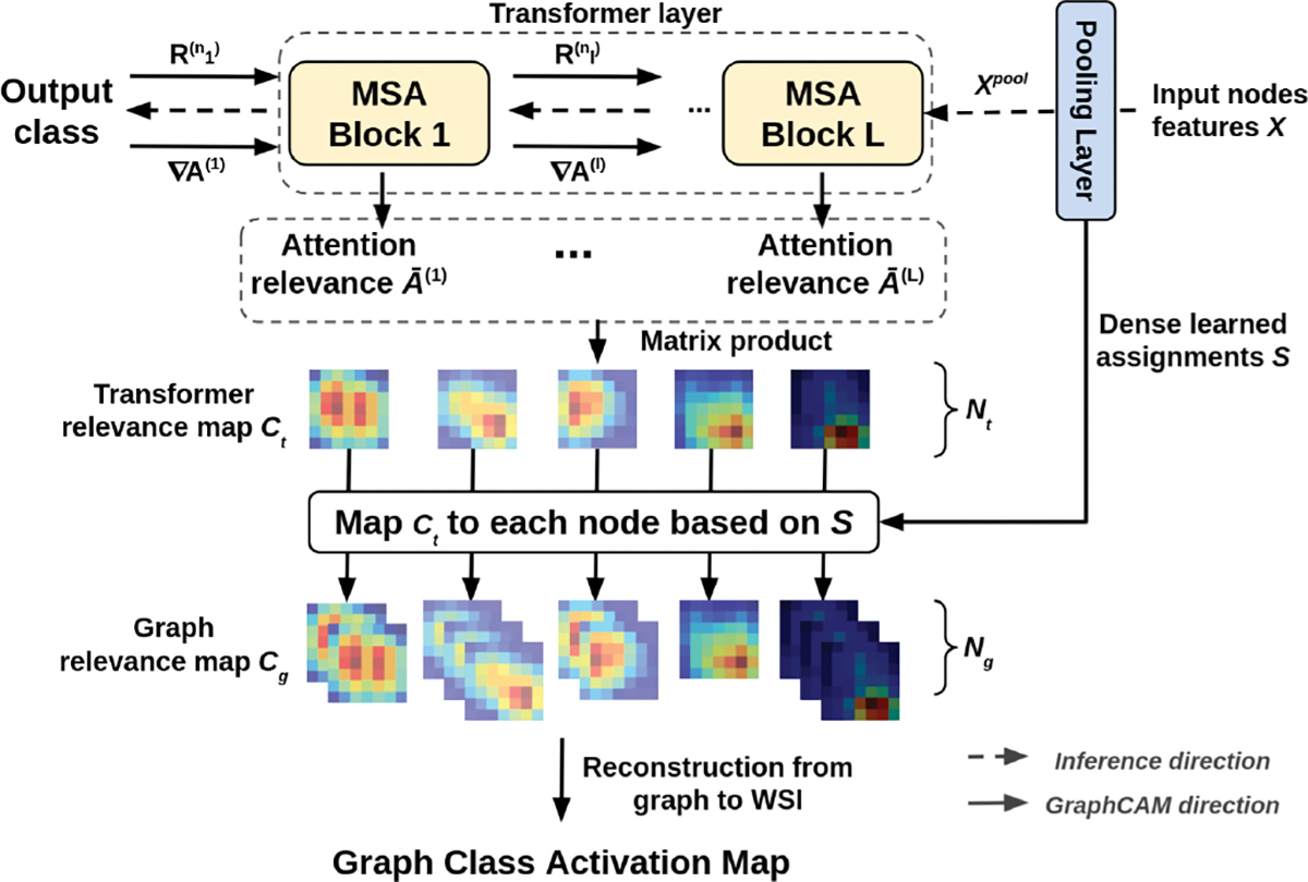
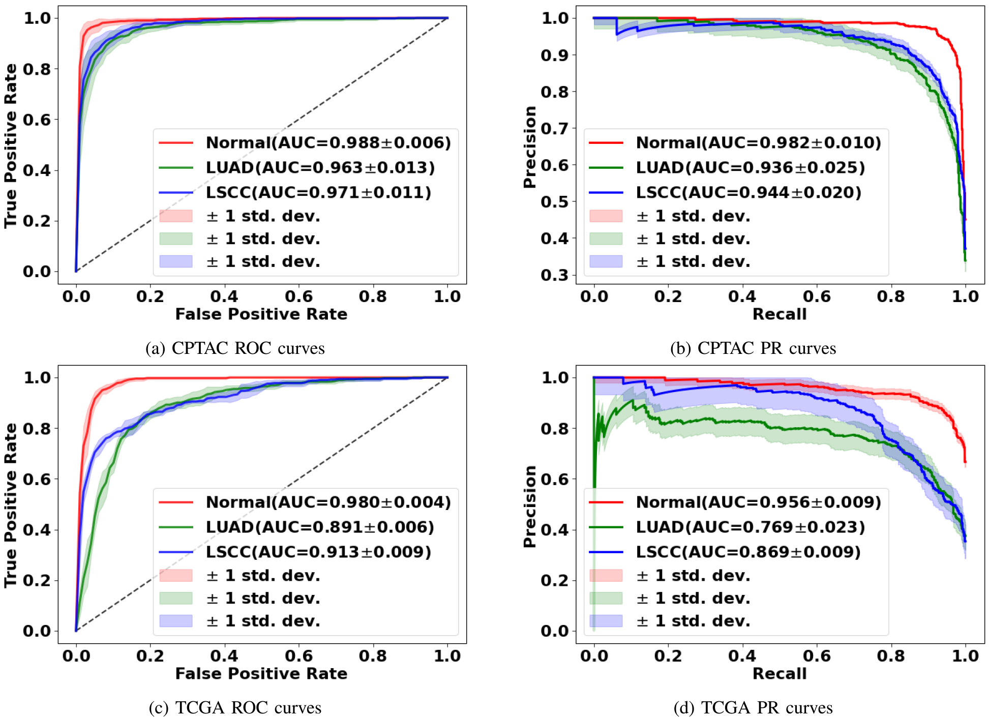
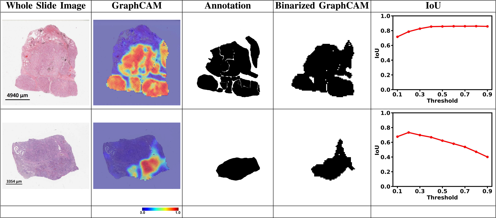
Verification
Claims the paper makes
The claims and statistics of this paper haven’t been checked yet.
Run the check — free, no account needed. It reads the open-access text and checks the sources it cites.
Claims other papers make about this one
Each is checked against this paper’s own text: does it say what the citing paper says it does?
In the citing paper
“While other researchers have previously explored the development of mid-level-fusion and mixer architectures [6], [7] as well as the use of graph-based representations of WSIs [8], our work is unique in mixing node and edge embeddings along with fusion of bulk gene expression embeddings to learn a multimodal topographic mapping to predict survival.”
From Graph attention-based fusion of pathology images and gene expression for prediction of cancer survival (2024) · cites this paper as [8]
In the citing paper
“We used NLST for generating node-level features for graph construction [8], TCGA for training the models using 5-fold cross-validation, and CPTAC as an independent dataset for testing.”
From Graph attention-based fusion of pathology images and gene expression for prediction of cancer survival (2024) · cites this paper as [8]
In the citing paper
“The ISM model’s performance exceeded that of other recent methodologies [8], [21], [25]-[27], as illustrated in Table II.”
From Graph attention-based fusion of pathology images and gene expression for prediction of cancer survival (2024) · cites this paper as [8]
Self-check
Percentages, sums and reported differences re-computed from the paper’s own numbers.
The self-check needs the paper’s full text.
Citations
Cites
Deep Residual Learning for Image Recognition
He, K., Zhang, X., Ren, S., & Sun, J. (2016) · 2016 IEEE Conference on Computer Vision and Pattern Recognition (CVPR) · doi:10.1109/cvpr.2016.90 · Cited by 235,474
Vaswani, A., Shazeer, N., Parmar, N., Uszkoreit, J., Jones, L., Gomez, A. N., Kaiser, L., & Polosukhin, I. (2017) · arXiv · doi:10.48550/arxiv.1706.03762 · Cited by 120,404
Adam: A Method for Stochastic Optimization
Kingma, D. P., & Ba, J. (2014) · arXiv · doi:10.48550/arxiv.1412.6980 · Cited by 98,946
ImageNet: A large-scale hierarchical image database
Deng, J., Dong, W., Socher, R., Li, L.-J., Li, K., & Fei-Fei, L. (2009) · 2009 IEEE Conference on Computer Vision and Pattern Recognition · doi:10.1109/cvpr.2009.5206848 · Cited by 65,333
Semi-supervised classification with graph convolutional networks
Kipf, T. N., & Welling, M. (2016) · arXiv · doi:10.48550/arxiv.1609.02907 · Cited by 24,853
Reduced Lung-Cancer Mortality with Low-Dose Computed Tomographic Screening
The National Lung Screening Trial Research Team (2011) · New England Journal of Medicine · doi:10.1056/nejmoa1102873 · Cited by 11,064
A simple framework for contrastive learning of visual representations
Chen, T., Kornblith, S., Norouzi, M., & Hinton, G. (2020) · arXiv · doi:10.48550/arxiv.2002.05709 · Cited by 10,857
Deformable DETR: Deformable Transformers for End-to-End Object Detection
Zhu, X., Su, W., Lu, L., Li, B., Wang, X., & Dai, J. (2020) · arXiv · doi:10.48550/arxiv.2010.04159 · Cited by 6,027 · cited 1×
“row normalization function in transformers for computer vision tasks [36], [37].”
BackgroundSGDR: Stochastic Gradient Descent with Warm Restarts
Loshchilov, I., & Hutter, F. (2016) · arXiv · doi:10.48550/arxiv.1608.03983 · Cited by 5,309
TransUNet: Transformers Make Strong Encoders for Medical Image Segmentation
Chen, J., Lu, Y., Yu, Q., Luo, X., Adeli, E., Wang, Y., Lu, L., Yuille, A. L., & Zhou, Y. (2021) · arXiv · doi:10.48550/arxiv.2102.04306 · Cited by 4,206
Research works printed but not linked: 2
- Dosovitskiy, An image is worth 16×16 words: Transformers for image recognition at scale
- 2021, The Cancer Genome Atlas Program
Cited by
Sorted by citations
Items 201–255 of 255
Yu, H., Diao, Y., Liu, X., Wang, H., Zhu, J., Gao, J., & Pedrycz, W. (2025) · Information Sciences · doi:10.1016/j.ins.2025.122843
Ding, X., Li, H., Tang, Y., Lang, X., Lv, W., He, B., & Ma, Y. (2025) · Physics in Medicine and Biology · doi:10.1088/1361-6560/ae19c6 · Cited by 1
Adaptive Multi-Scale Graph Transformer Framework for Histopathological Images
Wu, C.-I., Banda, K., Swisher, E. M., & Sailem, H. (2026) · IEEE International Symposium on Biomedical Imaging (ISBI) · doi:10.1109/isbi61048.2026.11515631
“Frameworks such as HIPT [10], H 2 -MIL [11], and MS-RGCN [12] integrate cellular-and tissue-level representations but incur substantial memory overhead due to dense cross-scale interactions.”
Duran, J., Zou, Y., Vallières, M., & Enger, S. A. (2025) · Machine Learning with Applications · doi:10.1016/j.mlwa.2025.100789
Luo, D., Liu, X., chu, X., Chen, J., Qi, M., Zuo, P., Li, S., & Wang, F. Y. (2025) · SSRN Electronic Journal · doi:10.2139/ssrn.5804592
Raseena, T. P., Balasundaram, S. R., & Kumar, J. (2025) · Computers & Electrical Engineering · doi:10.1016/j.compeleceng.2025.110867
Ali, H., Mohsen, F., & Shah, Z. (2024) · Figshare · doi:10.6084/m9.figshare.26617579
Ali, H., Mohsen, F., & Shah, Z. (2024) · Figshare · doi:10.6084/m9.figshare.26617582
Ali, H., Mohsen, F., & Shah, Z. (2024) · Figshare · doi:10.6084/m9.figshare.26617576
WSI-GT: Pseudo-Label Guided Graph Transformer for Whole-Slide Histology
Sun, Z., Khvostikov, A. V., Krylov, A. S., Mikhailov, I. А., & Malkov, P. G. (2025) · Machine Learning and Knowledge Extraction · doi:10.3390/make8010008
“Zheng et al. [11] utilized a Graph Transformer that combines a graph-based representation of a WSI with features from a vision transformer to predict disease grade, achieving high accuracy across various datasets.”
Wu, Y., Xie, X., Zhao, C., Song, P., Yin, F., Wu, G., & Yu, J. (2026) · IEEE Transactions on Image Processing · doi:10.1109/tip.2026.3654402
“Graph-based methods [3], [10], [19], [20] preserve spatial relationships between instances using graph structures, with recent innovations like TEA-Graph [3] introducing super-patches to improve computational e ffi ciency while maintaining representation quality.”
Dual‐Scale Transformer Fusion With Meta Learning for Micro Metastasis Detection in Thyroid Cancer
Wang, J., Shi, J., Ni, H., Zhao, L., Huang, J., & Li, J. (2026) · Advanced Intelligent Systems · doi:10.1002/aisy.202501397
“Transformers excel in pathological image analysis [57, 58] due to their patch-based self-attention, which captures both fine morphological and global contextual features.”
An End-to-end learning for classification and segmentation of breast cancer
Chen, J., Chen, J., Tan, Z., Tang, Z., Wei, J., Ke, Q., Ji, Y., & Gao, Z. (2026) · Multimedia Tools and Applications · doi:10.1007/s11042-026-21306-6
A Lightweight Transfer Learning Framework for Lung Cancer Detection from Histopathology Images
Jain, S., Pooja, Pal, A., & Dixit, A. (2025) · International Conference on Computing and Communications (COMPUTINGCON) · doi:10.1109/computingcon64838.2025.11376744
“According to authors [20][21][22], when applying the CNN models to new datasets from different institutions, the accuracy of the models was found to drop considerably, bringing attention to how important it is to develop effective ways for models to generalize.”
Tsang, A. P., Krishnan, S. R. A., Kulkarni, R., Bhadury, S., di Magliano, M. P., Frankel, T. L., & Rao, A. (2026) · npj Artificial Intelligence · doi:10.1038/s44387-026-00075-5
“5),learningrate(1e-5to1e-2),weightdecay (1e-6to1e-3),andbatchsize(16,32).”
Bai, X., Zhang, Y., Yuan, L., Li, R., Li, J., Fu, K., Li, X., & Li, C. (2025) · IEEE International Conference on Big Data (BigData) · doi:10.1109/bigdata66926.2025.11401946
“The Graph-Transformer (GT) model introduced a graph-based saliency mapping method, enhancing the interpretability of whole slide image classification while maintaining efficient inference [27].”
Ji, H., Lei, Y., Sun, M., & Zhang, T. (2025) · International Conference on Virtual Reality and Visualization · doi:10.1109/icvrv67992.2025.00054
“GTMIL [23] combined graph-based WSI representations with Transformer to better capture inter-instance correlations.”
InfluentialYang, J., Pang, X., Lin, C., & Tan, T. (2026) · Expert Systems with Applications · doi:10.1016/j.eswa.2026.132123
Context aware deep learning techniques for analysis of breast cancer histopathology: a review
Dutta, R. M., Sekh, A. A., Dogra, D. P., & Dan, P. K. (2026) · Discover Computing · doi:10.1007/s10791-026-10071-7
MorphoNet: Morphological sub-region-based structure learning for WSI analysis
Wang, F., Wu, F., Hu, M., He, J., Wang, L., Chen, J., Liang, L., Wang, S., & Yu, L. (2026) · Medical Image Analysis · doi:10.1016/j.media.2026.104061
Graph Neural Representations of Mammographic Images for Explainable Breast Cancer Detection
Pelluet, G. (2024) · theses.fr (ABES) · doi:10.70675/3f96a5b0z6ccaz46f9za2efz26ce24b16577
A histopathology image–based computer-aided classification study for oral squamous cell carcinoma
任益萍, Li, R., & Chen, D. (2026) · Frontiers in Oncology · doi:10.3389/fonc.2026.1806332
Kong, C., Guan, Y., Li, C. S., Chen, P., Liu, L., & Lin, Y. (2026) · IEEE International Conference on Acoustics Speech and Signal Processing · doi:10.1109/icassp55912.2026.11460328
Chanda, D., Yahyasoltani, N., & Ganji, M. (2026) · IEEE International Conference on Acoustics Speech and Signal Processing · doi:10.1109/icassp55912.2026.11463619
SLDPC: Slide-Level Dual-Prompt Collaboration for few-shot whole slide image classification
Yuan, L., Zheng, Y., Liu, W., Zhao, H., Zhang, W., Wei, B., & Chen, L. (2026) · Computerized Medical Imaging and Graphics · doi:10.1016/j.compmedimag.2026.102768
Self-citationA Review on Deep Learning and Interpretable AI Techniques for the Detection of Lung and Colon Cancer
Anusha, N., & Mahanty, C. (2026) · Communications in computer and information science · doi:10.1007/978-3-032-16830-6_11
Gao, G., Zhang, K., Hu, D., Gan, T., Yang, J., & Rao, N. (2026) · Information Processing & Management · doi:10.1016/j.ipm.2026.104846
Xie, H., Xu, T., Yang, H., Lyu, M., Chen, C. Y., Tong, C., & Liu, S. (2026) · Computer Methods and Programs in Biomedicine · doi:10.1016/j.cmpb.2026.109407
Ramanathan, V., Xu, T., Pati, P., Ahmed, F., Goubran, M., & Martel, A. L. (2025) · IEEE/CVF International Conference on Computer Vision (ICCV) · doi:10.1109/iccv51701.2025.02217 · Cited by 3
“Multiple Instance Learning (MIL) has become a key method for WSI analysis, dividing WSIs into patches, extracting features using pre-trained models, and aggregating them into slide-level representations through various pooling methods [10, 29, 54, 59, 61, 79].”
Lee, B. H., Jeong, W., Han, W., Lee, K., & Chun, S. Y. (2025) · IEEE/CVF International Conference on Computer Vision (ICCV) · doi:10.1109/iccv51701.2025.02157
“Multiple instance learning (MIL) [7, 12, 24, 33, 34, 39, 41, 56, 58, 72, 74, 76] is a promising approach to mitigate high annotation costs by utilizing only bag-level (or slide-level) weak labels for large-scale images like histopathological whole slide images (WSIs).”
Bai, W., Zhang, Y., Guo, Q., Liu, W., Ning, Z., Cheng, S., Yang, C. R., & Song, L. (2026) · IEEE Transactions on Intelligent Transportation Systems · doi:10.1109/tits.2026.3689136
“Graph Transformers e ff ectively integrate Transformer architectures with GNNs [46], [47], [48], achieving success in fields ranging from computer vision [49], [50] to drug discovery [51], [52] and social network analysis [53].”
Ghafour, B. A., & Ali, A. M. (2026) · ARO-The Scientific Journal of Koya University · doi:10.14500/aro.12768
Wu, J., Zhao, C., Yuan, J., Zhou, Q., Wei, Y., Li, J., Edzeafene-Mensah, E., Wang, O., Yang, C., Wang, M., et al. (2026) · Computerized Medical Imaging and Graphics · doi:10.1016/j.compmedimag.2026.102788
Multimodal information compression, completion, and adaptive fusion for cancer survival prediction
Gao, G., Gan, T., Yang, J., & Rao, N. (2026) · Information Fusion · doi:10.1016/j.inffus.2026.104548
Liang, M., Wang, X., Li, B., Zhang, Y., Zhang, Y., Jia, X., & Wang, L. (2026) · IEEE Transactions on Pattern Analysis and Machine Intelligence · doi:10.1109/tpami.2026.3702808
AGE-MIL: Anchor-Guided Evidence Learning for Patient-Level Prediction
Niu, J., (15340), J. C., Zhang, D., Lu, J., Liao, Z., Liu, X., Zhong, H., Crispin-Ortuzar, M., Li, C., Gao, Z., et al. (2026) · Lecture notes in computer science · doi:10.1007/978-3-032-38224-5_2
Lou, J., Pan, Q., Yang, Q., Yang, G., Ji, B., & Li, S. (2026) · IEEE Transactions on Circuits and Systems for Video Technology · doi:10.1109/tcsvt.2026.3708293
“Graph neural networks (GNNs) have gained significant attention for capturing topological structure, contextual information, relation information, and interactions for histopathology image classification [30], [31], [32], [33].”
InfluentialXiong, J., Zhu, Z., Gu, W., Li, Y. C., Zhao, M. L., Cai, J., Sun, C., Wang, J., & Yu, G. (2026) · World Journal of Pediatric Surgery · doi:10.1136/wjps-2025-001149
“Our strong performance on biopsy specimens, which often present with the highest diagnostic uncertainty, validates the clinical value of addressing this specific bottleneck first.”
Chen, X., Zhao, J., Peng, K., Wang, J., Mu, D., & Xu, H. (2026) · Engineering Applications of Artificial Intelligence · doi:10.1016/j.engappai.2026.115665
Chen, T., Xiaoyu, L., Xu, J., Hua, Y., Zhang, H., Yang, B., & Xia, Q. (2026) · Engineering Applications of Artificial Intelligence · doi:10.1016/j.engappai.2026.115630
Hu, H., Wang, S., Xiao, Y., Yu, H., Fang, Z., Han, L. S., & Li, Y. (2026) · Lecture notes in computer science · doi:10.1007/978-981-92-3513-1_42
Gao, Y., Ma, T., Li, L., Ding, Y., Qi, R., Cui, X., & Gao, X. (2026) · Chinese Medical Journal · doi:10.1097/cm9.0000000000004154
Kunzmann, M., Elizondo-Cantú, M. C., Bischofs, I. B., & Rohr, K. (2026) · Medical Image Analysis · doi:10.1016/j.media.2026.104275
Ahad, M. T., & Payel, I. J. (2026) · Neural Computing and Applications · doi:10.1007/s00521-026-12414-3
Spatial–frequency graph attention network for predicting HER2 status in breast cancer histopathology
Xie, H., Zhuang, J., Long, Q., Zeng, J., Yang, M., Zhai, Y., Huang, H., & Qin, C. (2026) · Biomedical Signal Processing and Control · doi:10.1016/j.bspc.2026.111335
Artificial Intelligence for Thyroid Histopathology Image Analysis: A Systematic Review
Tao, G., Yaakob, R., & Abdipoor, S. (2026) · Journal of Artificial Intelligence · doi:10.3923/jai.2026.78.93
A Gradient-Level Diagnosis of Extreme Class Imbalance in Multiple Instance Learning via q-Calculus
Rehman, A. A., Baro, E. N., & Otero, P. (2026) · Machine Learning and Knowledge Extraction · doi:10.3390/make8090282
Liu, L., & Wei, W. (2026) · Journal of King Saud University - Computer and Information Sciences · doi:10.1007/s44443-026-01286-1
AceMIL: Ordinal-Aware Multiple Instance Learning for Pathological Progression Analysis
Li, S., Chen, Y., Gong, Y., Zhou, H., Chen, F.-J., Gao, X., & Chen, Z. (2026) · doi:10.1109/cvprf71909.2026.00513
“Recent MIL methods have achieved remarkable progress through attention-based aggregation [18, 45], self-supervised pretraining [6, 20, 35], graph-based reasoning [25, 62], and other architectural innovations [19, 23, 27, 48, 58, 60].”
CSNet: Cognitive Simulation Network for Reliable Histopathology-Based Cancer Diagnosis
Zhu, Y., Wang, X., Su, S., Guo, M., Tao, T., & Dai, Y. (2026) · Journal of Imaging Informatics in Medicine · doi:10.1007/s10278-026-02388-y
CytoSet: Bethesda-order-aware set prediction for cervical cytology cell detection
He, C., Chen, F., Zheng, H., Guo, W., Chen, Z., Yang, C., Fang, B., Zhou, Q., & Fang, B. (2026) · Neurocomputing · doi:10.1016/j.neucom.2026.135398
Bhuvanya, R., Thandapani, S., Iqbal, M. M., & Adikrishanan, S. (2026) · Discover Artificial Intelligence · doi:10.1007/s44163-026-02437-z
FPAL: a full-process probability-driven active learning for whole slide image diagnosis
Xu, Z., Cai, Y., Han, T., Jia, X., Xu, W., & Yang, N. (2026) · Pattern Analysis and Applications · doi:10.1007/s10044-026-01792-y
Zhao, X., Yang, Y., Lai, Z., Huang, Y., Hou, J., Zhang, R., Lin, Z., Qu, Z., & Qin, W. (2026) · The Innovation Informatics · doi:10.59717/j.xinn-inform.2026.100065
Metadata
- Authors
- Zheng, Y., Gindra, R. H., Green, E. J., Burks, E. J., Betke, M., Beane, J. E., & Kolachalama, V. B.
- Affiliations
- Boston University (US)
- ORCID
- Venue
- IEEE Transactions on Medical Imaging
- Published
- 2022-11
- Volume
- 41
- Issue
- 11
- Pages
- 3003-3015
- ISSN
- 0278-0062 (ISSN-L)
- 1558-254X
- PMC
- PMC9670036
- OpenAlex
- W4281257868
- Cited by
- 255
- References
- 47
- Citations by year
- 2026: 54 · 2025: 81 · 2024: 73 · 2023: 42 · 2022: 5
- FWCI
- 16.55
- Type
- journal article
- Language
- en
- Open access
- hybrid
- doi.org
- Licence
- Locations
- IEEE Transactions on Medical Imaging (publishedVersion, cc-by)
- medRxiv (acceptedVersion, cc-by)
- PubMed (publishedVersion)
- PubMed Central (acceptedVersion, cc-by)
- arXiv (Cornell University) (submittedVersion)
- arXiv (Cornell University) (cc-by)
- Funders
- Grants from the National Institutes of Heath (R21-CA253498, R01-HL159620)
- Johnson & Johnson Enterprise Innovation, Inc.
- American Heart Association (20SFRN35460031)
- Karen Toffler Charitable Trust
- National Science Foundation (1551572, 1838193)
- Topics
- Physical Sciences › Computer Science › Artificial Intelligence › AI in cancer detection
- Health Sciences › Medicine › Radiology, Nuclear Medicine and Imaging › Radiomics and Machine Learning in Medical Imaging
- Physical Sciences › Computer Science › Computer Vision and Pattern Recognition › Advanced Neural Network Applications
- Keywords
- whole slide image classification, graph transformer, vision transformer, lung adenocarcinoma, squamous cell carcinoma, lung cancer histopathology, contrastive learning, interpretability
- MeSH terms
- Guanosine Triphosphate, Image Processing, Computer-Assisted, Proteomics
About these checks
Registry, retraction, Cites and statistics results are computed, not judged, with one exception: a printed reference that no index lists is read once by a model before it counts as a citation error. Claims are extracted by a model and kept only when their quote appears verbatim in the text; each cited source is then checked, with a model’s help, for whether it says what the claim relies on. Those verdicts can be wrong — read the claim’s quote and the cited source before relying on one.
Statistics and arithmetic are recomputed, not judged.
Confidence bands are shown only for fields calibrated on our annotated test set. None is calibrated yet, so no band is shown.
What counts as a claim ›How we measure confidence ›How we check this ›
Are you an author, or do you see a problem with this page? Request a review
