

The DOI matches its Crossref record; 12 of the 12 references it cites were found in a registry or an index.
Using Chao’s Estimator as a Stopping Criterion for Technology-Assisted Review
Abstract
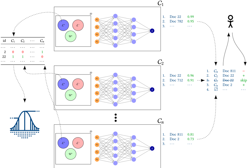
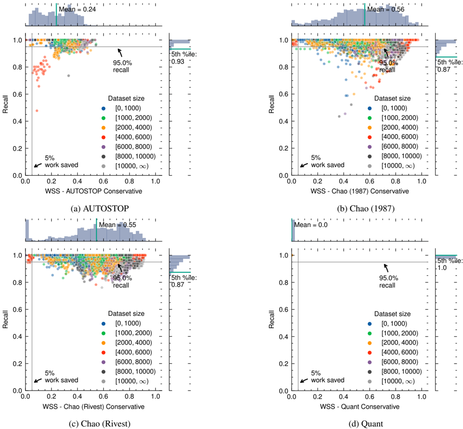
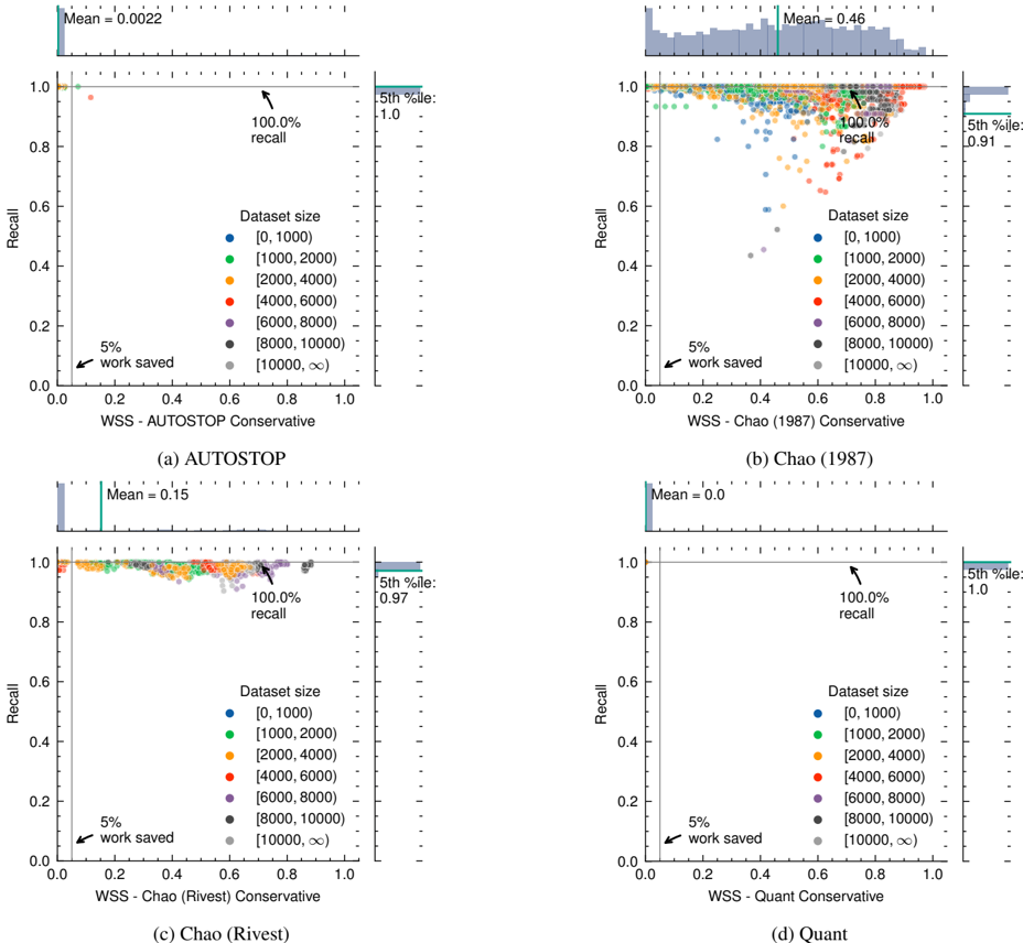
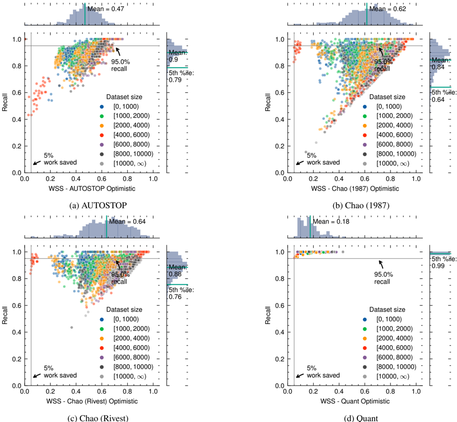
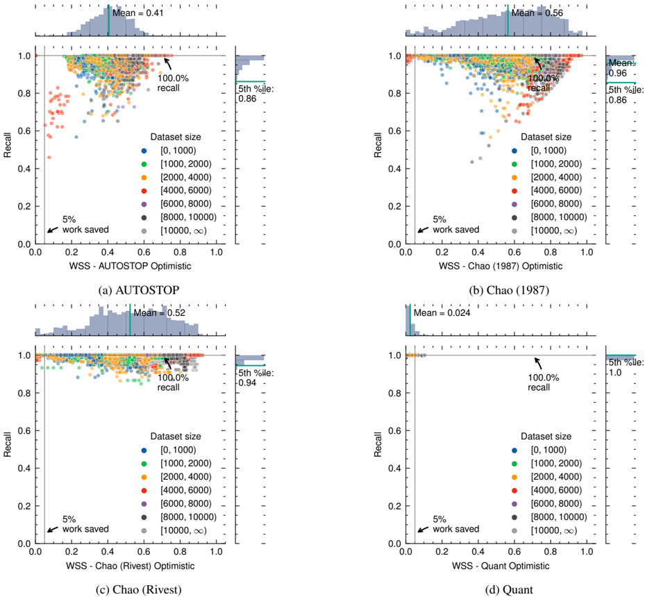
Technology-Assisted Review aims to reduce the human effort required for screening processes such as abstract screening for Systematic Literature Reviews. Human reviewers label documents as relevant or irrelevant during this process, while the system incrementally updates a prediction model based on the reviewers’ previous decisions. After each model update, the system proposes new documents it deems relevant, to prioritize relevant documents over irrelevant ones. A stopping criterion is necessary to guide users in stopping the review process to minimize the number of missed relevant documents and the number of read irrelevant documents. In this article, we propose and evaluate a new ensemble-based Active Learning strategy and a stopping criterion based on Chao’s Population Size Estimator that estimates the prevalence of relevant documents in the dataset. Our simulation study demonstrates that this criterion performs well on several datasets and is compared to other methods presented in the literature.
Overview
The claims and statistics of this paper haven’t been checked yet.
Run the check — free, no account needed. It reads the open-access text and checks the sources it cites.
Integrity signals
Registry
Cites
Statistics
Figures
Verification
Claims the paper makes
The claims and statistics of this paper haven’t been checked yet.
Run the check — free, no account needed. It reads the open-access text and checks the sources it cites.
Claims other papers make about this one
Each is checked against this paper’s own text: does it say what the citing paper says it does?
In the citing paper
“The number of missed records depends, in effect, on the stopping rule and the model's performance in identifying the final relevant records [6].”
From Large-scale simulation study of active learning models for systematic reviews (2025) · cites this paper as [6]
In the citing paper
“In the current active learning pipeline, some dataset segments go unscreened when the dataset appears sufficiently sparse, and the stopping rule is reached [6].”
From Large-scale simulation study of active learning models for systematic reviews (2025) · cites this paper as [6]
Self-check
Percentages, sums and reported differences re-computed from the paper’s own numbers.
The self-check needs the paper’s full text.
Citations
Cites
An open source machine learning framework for efficient and transparent systematic reviews
van de Schoot, R., de Bruin, J., Schram, R., Zahedi, P., de Boer, J., Weijdema, F., Kramer, B., Huijts, M., Hoogerwerf, M., Ferdinands, G., et al. (2021) · Nature Machine Intelligence · doi:10.1038/s42256-020-00287-7 · Cited by 1,157
Reducing Workload in Systematic Review Preparation Using Automated Citation Classification
Cohen, A. M., Hersh, W. R., Peterson, K., & Yen, P.-Y. (2006) · Journal of the American Medical Informatics Association · doi:10.1197/jamia.m1929 · Cited by 411 · cited 1×
“5 with a target recall of 95 %.”
Chai, K. E. K., Lines, R. L. J., Gucciardi, D. F., & Ng, L. (2021) · Systematic Reviews · doi:10.1186/s13643-021-01635-3 · Cited by 190 · cited 2×
“Recently, systems were proposed and built that potentially reduce the human effort needed by limiting the number of irrelevant documents shown to the reviewer [9, 15, 37, 43].”
Shemilt, I., Simon, A., Hollands, G. J., Marteau, T. M., Ogilvie, D., O'Mara‐Eves, A., Kelly, M. P., & Thomas, J. (2014) · Research Synthesis Methods · doi:10.1002/jrsm.1093 · Cited by 170
Statistical stopping criteria for automated screening in systematic reviews
Callaghan, M. W., & Müller-Hansen, F. (2020) · Systematic Reviews · doi:10.1186/s13643-020-01521-4 · Cited by 121 · cited 26×
“The Poisson parameter can vary for each document i , allowing for heterogeneity in capture probabilities.”
InfluentialEngineering Quality and Reliability in Technology-Assisted Review
Cormack, G. V., & Grossman, M. R. (2016) · Proceedings of the 39th International ACM SIGIR conference on Research and Development in Information Retrieval · doi:10.1145/2911451.2911510 · Cited by 98
Virus Metagenomics in Farm Animals: A Systematic Review
Kwok, K. T. T., Nieuwenhuijse, D. F., Phan, M. V. T., & Koopmans, M. P. G. (2020) · Viruses · doi:10.3390/v12010107 · Cited by 97
FAST2: An intelligent assistant for finding relevant papers
Yu, Z., & Menzies, T. (2019) · Expert Systems with Applications · doi:10.1016/j.eswa.2018.11.021 · Cited by 80
Active learning for screening prioritization in systematic reviews - A simulation study
Ferdinands, G., Schram, R., de Bruin, J., Bagheri, A., Oberski, D. L., Tummers, L., & van de Schoot, R. (2020) · doi:10.31219/osf.io/w6qbg · Cited by 51
Kastner, M., Straus, S. E., McKibbon, K. A., & Goldsmith, C. H. (2009) · Journal of Clinical Epidemiology · doi:10.1016/j.jclinepi.2008.06.001 · Cited by 47
SYNERGY - Open machine learning dataset on study selection in systematic reviews
De Bruin, J., Ma, Y., Ferdinands, G., Teijema, J., & Van de Schoot, R. (2023) · DataverseNL · doi:10.34894/he6naq · Cited by 20
Capture-mark-recapture to estimate the number of missed articles for systematic reviews in surgery
Stelfox, H. T., Foster, G., Niven, D., Kirkpatrick, A. W., & Goldsmith, C. H. (2013) · The American Journal of Surgery · doi:10.1016/j.amjsurg.2012.11.017 · Cited by 9
Research works printed but not linked: 38
- 10.5555/69372 · DOI
- 10.1007/BF01002566 · DOI
- 10.18637/jss.v019.i05 · DOI
- 10.1007/s10651-020-00440-w · DOI
- 10.4324/9781315151939 · DOI
- 10.1093/biomet/65.3.625 · DOI
- 10.2307/1936861 · DOI
- 10.2307/2531532 · DOI
- 10.1002/0471667196.ess5051 · DOI
- 10.2436/20.8080.02.49 · DOI
- Carl V. L. Charlier. 1905. Die zweite form des fehlergesetzes. Meddelanden Fran Lunds Astronomiska Observatorium Serie I 26 (1905), 1–8.
- 10.1016/j.ejor.2005.06.023 · DOI
- Gordon V. Cormack and Maura R. Grossman. 2015. Autonomy and reliability of continuous active learning for technology-assisted review. arXiv:1504.06868. Retrieved from https://arxiv.org/abs/1504.06868 · arXiv
- Gordon V. Cormack and Maura R. Grossman. 2017. Technology-assisted review in empirical medicine: Waterloo participation in CLEF eHealth 2017. In Working Notes of CLEF 2017; Conference and Labs of the Evaluation Forum (CEUR Workshop Proceedings, Vol. 1866), Linda Cappellato, Nicola Ferro, Lorraine Goeuriot, and Thomas Mandl (Eds.), CEUR-WS.org.
- 10.2307/2532310 · DOI
- A. W. F. Edwards. 1972. Likelihood: An Account of the Statistical Concept of Likelihood and Its Application to Scientific Inference. University Press, Cambridge [Eng.].
- 10.2307/2987516 · DOI
- 10.1109/ICDAR.1995.598994 · DOI
- 10.1002/0471715816 · DOI
- Evangelos Kanoulas, Dan Li, Leif Azzopardi, and Rene Spijker. 2017. CLEF 2017 technologically assisted reviews in empirical medicine overview. CEUR Workshop Proceedings 1866 (2017), 1–29.
- Evangelos Kanoulas, Dan Li, Leif Azzopardi, and Rene Spijker. 2018. CLEF 2018 technologically assisted reviews in empirical medicine overview: 19th working notes of CLEF conference and labs of the evaluation forum, CLEF 2018. CEUR Workshop Proceedings 2125 (2018), 1–34.
- Evangelos Kanoulas, Dan Li, Leif Azzopardi, and Rene Spijker. 2019. CLEF 2019 technology assisted reviews in empirical medicine overview. CEUR Workshop Proceedings 2380 (2019), 9–12.
- Guolin Ke, Qi Meng, Thomas Finley, Taifeng Wang, Wei Chen, Weidong Ma, Qiwei Ye, and Tie-Yan Liu. 2017. LightGBM: A highly efficient gradient boosting decision tree. In Advances in Neural Information Processing Systems. I. Guyon, U. Von Luxburg, S. Bengio, H. Wallach, R. Fergus, S. Vishwanathan, and R. Garnett (Eds.), Vol. 30. Curran Associates, Inc, 3149–3157.
- 10.1126/science.abl7655 · DOI
- 10.1186/1471-2288-14-58 · DOI
- 10.1145/3459637.3482415 · DOI
- 10.1145/3411755 · DOI
- 10.1016/j.cegh.2023.101485 · DOI
- 10.1201/b17222 · DOI
- 10.1111/j.1541-0420.2007.00779.x · DOI
- 10.1016/j.jclinepi.2011.03.008 · DOI
- 10.1145/130385.130417 · DOI
- 10.1111/1467-9574.00232 · DOI
- Byron C. Wallace, Issa J. Dahabreh, Kelly H. Moran, Carla E. Brodley, and Thomas A. Trikalinos. 2013. Active literature discovery for scoping evidence reviews. In KDD Workshop on Data Mining for Healthcare (KDDDMH’13), 14–19.
- 10.1080/00031305.2013.783881 · DOI · Paper page
- 10.1145/3477495.3531663 · DOI
- 10.1145/3469096.3469873 · DOI
- 10.1007/978-3-030-99736-6_34 · DOI
Cited by
ASReview LAB v.2: Open-source text screening with multiple agents and a crowd of experts
de Bruin, J., Lombaers, P., Kaandorp, C., Teijema, J., van der Kuil, T., Yazan, B., Dong, A., & van de Schoot, R. (2025) · Patterns · doi:10.1016/j.patter.2025.101318 · Cited by 27
Large-scale simulation study of active learning models for systematic reviews
Teijema, J. J., de Bruin, J., Bagheri, A., & van de Schoot, R. (2025) · International Journal of Data Science and Analytics · doi:10.1007/s41060-025-00777-0 · Cited by 13
Metadata
- Authors
- Bron, M., van der Heijden, P. G. M., Feelders, A., & Siebes, A.
- Venue
- ACM Transactions on Information Systems
- Published
- 2025-05-09
- Volume
- 43
- Issue
- 3
- Pages
- 1-51
- ISSN
- 1046-8188
- 1558-2868
- Cited by
- 7
- References
- 12
- Language
- en
About these checks
Registry, retraction, Cites and statistics results are computed, not judged, with one exception: a printed reference that no index lists is read once by a model before it counts as a citation error. Claims are extracted by a model and kept only when their quote appears verbatim in the text; each cited source is then checked, with a model’s help, for whether it says what the claim relies on. Those verdicts can be wrong — read the claim’s quote and the cited source before relying on one.
Statistics and arithmetic are recomputed, not judged.
Confidence bands are shown only for fields calibrated on our annotated test set. None is calibrated yet, so no band is shown.
What counts as a claim ›How we measure confidence ›How we check this ›
Are you an author, or do you see a problem with this page? Request a review
Data sources
Bibliographic data: Semantic Scholar, OpenAlex, Crossref.
Contains information from the Semantic Scholar Academic Graph Datasets, made available under the ODC Attribution License (ODC-BY 1.0).
Semantic Scholar’s data is described in: Kinney, R., et al. (2023). The Semantic Scholar Open Data Platform. arXiv:2301.10140.
