Student or educator? Sign up with your school email and get 6 months of Pro free.
Cited by 10

The DOI matches its Crossref record; 1 of the 1 references it cites were found in a registry or an index.

Analysis and Simulation of Intervention Strategies against Bus Bunching by means of an Empirical Agent‐Based Model

Quek, Wei Liang, Chung, Ning Ning, Saw, Vee-Liem, Chew, Lock Yue·2021·Complexity

Abstract

In this paper, we propose an empirically based Monte Carlo bus‐network (EMB) model as a test bed to simulate intervention strategies to overcome the inefficiencies of bus bunching. The EMB model is an agent‐based model which utilizes the positional and temporal data of the buses obtained from the Global Positioning System (GPS) to constitute (1) a set of empirical velocity distributions of the buses and (2) a set of exponential distributions of interarrival time of passengers at the bus stops. Monte Carlo sampling is then performed on these two derived probability distributions to yield the stochastic dynamics of both the buses’ motion and passengers’ arrival. Our EMB model is generic and can be applied to any real‐world bus network system. In particular, we have validated the model against the Nanyang Technological University’s Shuttle Bus System by demonstrating its accuracy in capturing the bunching dynamics of the shuttle buses. Furthermore, we have analyzed the efficacy of three intervention strategies: holding, no‐boarding, and centralized‐pulsing, against bus bunching by incorporating the rule set of these strategies into the model. Under the scenario where the buses have the same velocity, we found that all three strategies improve both the waiting and travelling times of the commuters. However, when the buses have different velocities, only the centralized‐pulsing scheme consistently outperforms the control scenario where the buses periodically bunch together.

Overview

The claims and statistics of this paper haven’t been checked yet.

Run the check — free, no account needed. It reads the open-access text and checks the sources it cites.

A few free checks a day · papers already verified open instantly · results are public

Integrity signals

Registry

Crossref · 10.1155/2021/2606191

Cites

1 of 1 references verified0 citation errors · 0 not checkable

Statistics

Figures

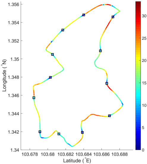
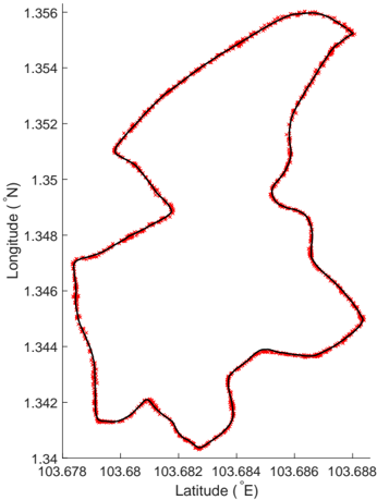
FIG. 1 Average velocity of the buses at different positions of the route. The path represents the 688 discretized positions of the route taken by NTU-SBS. The X and Y values represent actual GPS coordinates of the bus route. The color describes the average
FIG. 1 Average velocity of the buses at different positions of the route. The path represents the 688 discretized positions of the route taken by NTU-SBS. The X and Y values represent actual GPS coordinates of the bus route. The color describes the averageCC-BY · From the PDF
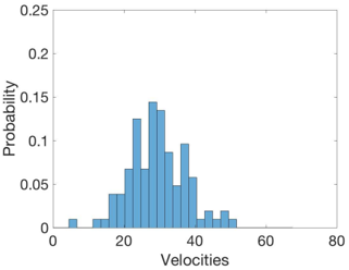
(a) Empirical distribution of velocities of the buses at position x = 542, which is the middle of a straight stretch of road.
(a) Empirical distribution of velocities of the buses at position x = 542, which is the middle of a straight stretch of road.CC-BY · From the PDF
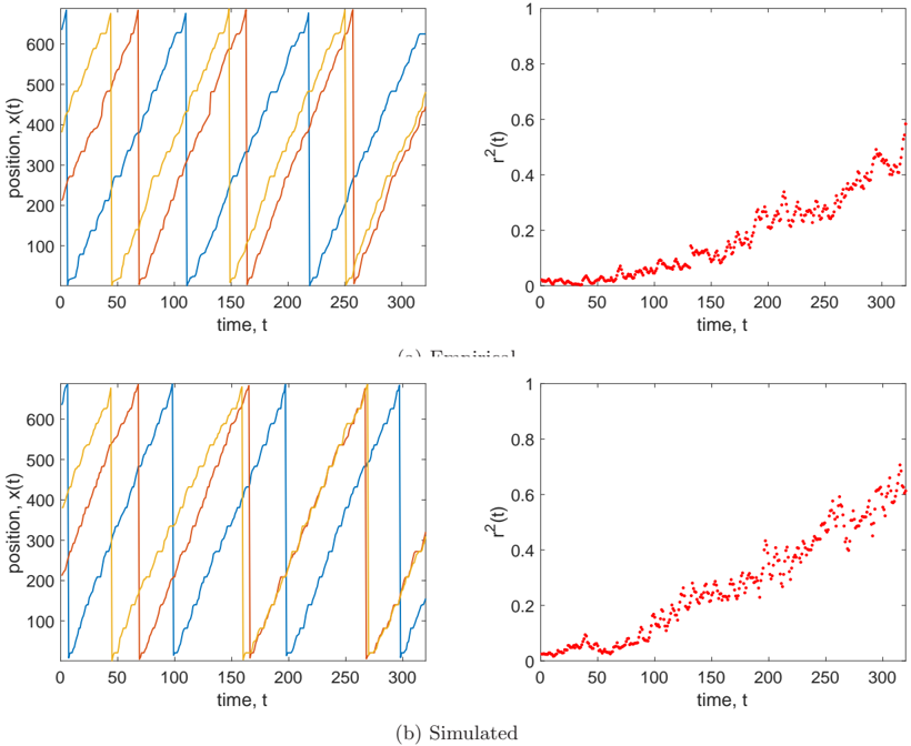
FIG. 3 Empirical trajectories of the three buses operating on 11 Sept 18, from 1404h - 1516h. The r 2 time series is derived from the trajectories and Eq. 2.
FIG. 3 Empirical trajectories of the three buses operating on 11 Sept 18, from 1404h - 1516h. The r 2 time series is derived from the trajectories and Eq. 2.CC-BY · From the PDF
FIG. 4 Plot of empirical and simulated trajectories. Each graph is selectively aggregated based on the initial r 2 of the trajectories from [ 0.0, 0.1 ) to [ 0.9, 1.0 ] . The statistical similarity between the empirical and simulated trajectories is tabulated in Table II
FIG. 4 Plot of empirical and simulated trajectories. Each graph is selectively aggregated based on the initial r 2 of the trajectories from [ 0.0, 0.1 ) to [ 0.9, 1.0 ] . The statistical similarity between the empirical and simulated trajectories is tabulated in Table IICC-BY · From the PDF
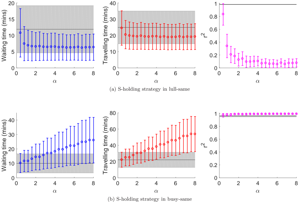
FIG. 5 Results of the s-holding strategy in the two same-velocity scenarios. Each colored point represents the mean and standard deviation of the measured quantities calculated from 100 realizations of each parameter value. The black line and grey shaded area of each graph denote the mean and standard deviation of the measured quantities from a control case, which are simulation runs of the same parameter values, without any intervention strategies.
FIG. 5 Results of the s-holding strategy in the two same-velocity scenarios. Each colored point represents the mean and standard deviation of the measured quantities calculated from 100 realizations of each parameter value. The black line and grey shaded area of each graph denote the mean and standard deviation of the measured quantities from a control case, which are simulation runs of the same parameter values, without any intervention strategies.CC-BY · From the PDF
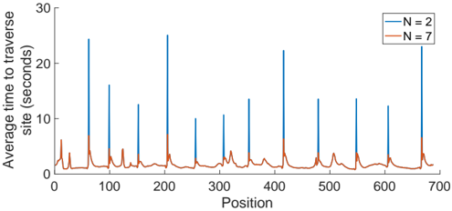
FIG. 6 The average time the bus takes to traverse each site of the route based on the number of active buses. The total time taken for a bus to reach its destination position can be derived by taking the total area under the curve between the two points.
FIG. 6 The average time the bus takes to traverse each site of the route based on the number of active buses. The total time taken for a bus to reach its destination position can be derived by taking the total area under the curve between the two points.CC-BY · From the PDF
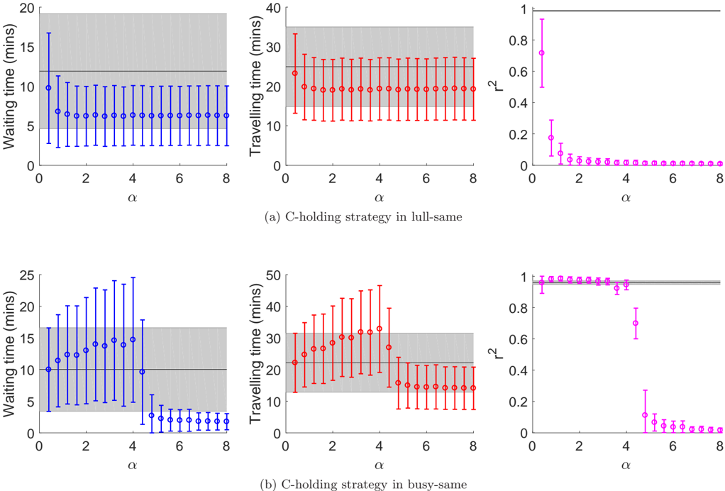
FIG. 7 Results of the c-holding strategy in the two same-velocity scenarios. Each colored point represents the mean and standard deviation of the measured quantities calculated from 100 realizations of each parameter value. The black line and grey shaded area of each graph denote the mean and standard deviation of the measured quantities from a control case, which are simulation runs of the same parameter values, without any intervention strategies.
FIG. 7 Results of the c-holding strategy in the two same-velocity scenarios. Each colored point represents the mean and standard deviation of the measured quantities calculated from 100 realizations of each parameter value. The black line and grey shaded area of each graph denote the mean and standard deviation of the measured quantities from a control case, which are simulation runs of the same parameter values, without any intervention strategies.CC-BY · From the PDF
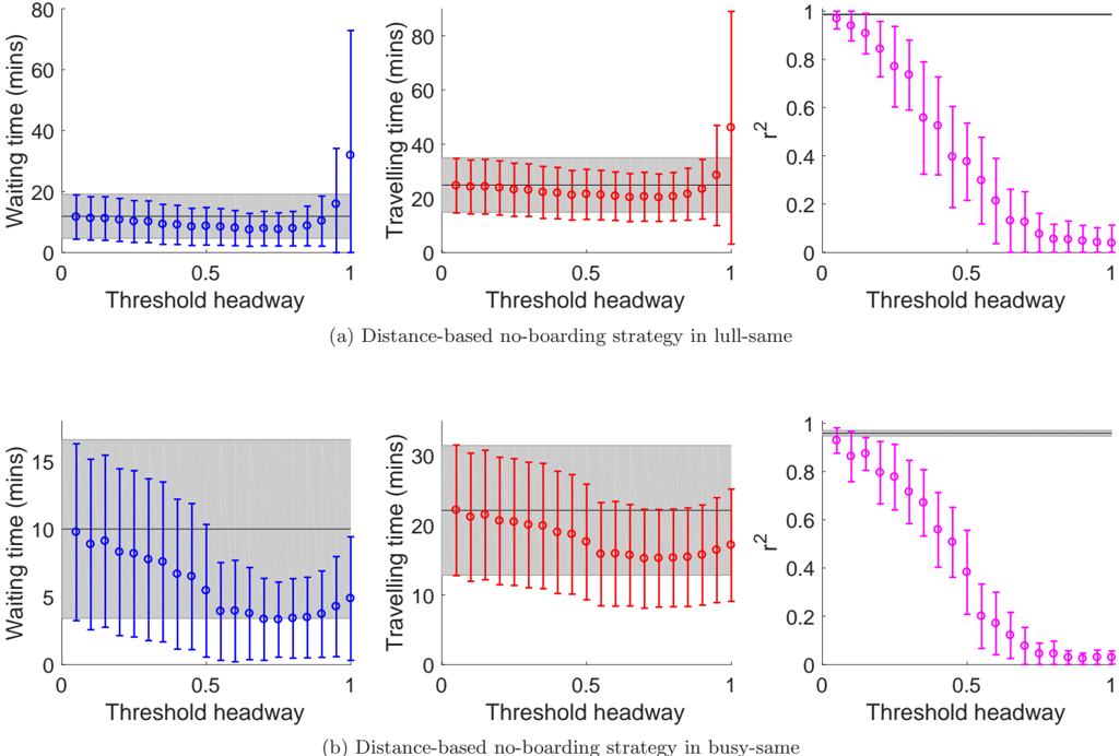
FIG. 8 Results of the distance-based no-boarding strategy on the two same-velocity scenarios. Each colored point represents the mean and standard deviation of the measured quantities calculated from 100 realizations of each parameter value. The black line and grey shaded area of each graph denote the mean and standard deviation of the measured quantities from a control case, which are simulation runs of the same parameter values, without any intervention strategies.
FIG. 8 Results of the distance-based no-boarding strategy on the two same-velocity scenarios. Each colored point represents the mean and standard deviation of the measured quantities calculated from 100 realizations of each parameter value. The black line and grey shaded area of each graph denote the mean and standard deviation of the measured quantities from a control case, which are simulation runs of the same parameter values, without any intervention strategies.CC-BY · From the PDF
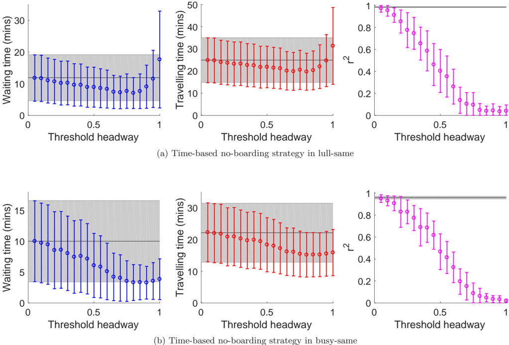
FIG. 9 Results of the time-based no-boarding strategy on the two same-velocity scenarios. Each colored point represents the mean and standard deviation of the measured quantities calculated from 100 realizations of each parameter value. The black line and grey shaded area of each graph denote the mean and standard deviation of the measured quantities from a control case, which are simulation runs of the same parameter values, without any intervention strategies.
FIG. 9 Results of the time-based no-boarding strategy on the two same-velocity scenarios. Each colored point represents the mean and standard deviation of the measured quantities calculated from 100 realizations of each parameter value. The black line and grey shaded area of each graph denote the mean and standard deviation of the measured quantities from a control case, which are simulation runs of the same parameter values, without any intervention strategies.CC-BY · From the PDF
Image 10
CC-BY · From the PDF
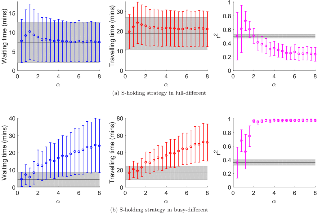
FIG. 11 Results of simulating the s-holding strategy in the two different-velocity scenarios. Each colored point represents the mean and standard deviation of the measured quantities calculated from 100 realizations of each parameter value. The black line and grey shaded area of each graph denote the mean and standard deviation of the measured quantities from a control case, which are simulation runs of the same parameter values, without any intervention strategies.
FIG. 11 Results of simulating the s-holding strategy in the two different-velocity scenarios. Each colored point represents the mean and standard deviation of the measured quantities calculated from 100 realizations of each parameter value. The black line and grey shaded area of each graph denote the mean and standard deviation of the measured quantities from a control case, which are simulation runs of the same parameter values, without any intervention strategies.CC-BY · From the PDF
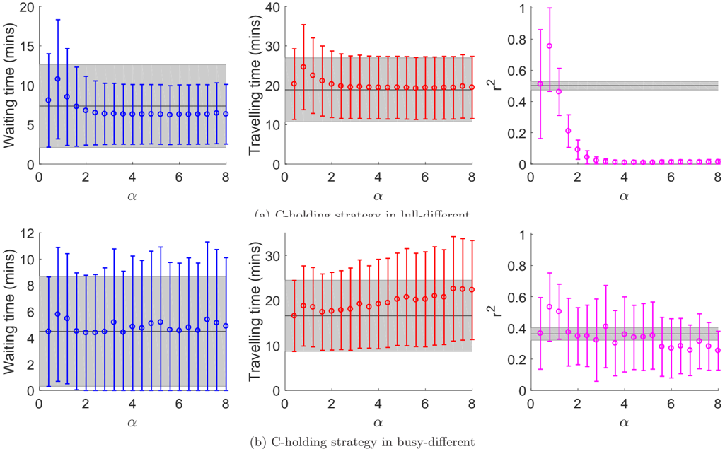
FIG. 12 Results of the c-holding strategy in the two different-velocity scenarios. Each colored point represents the mean and standard deviation of the measured quantities calculated from 100 realizations of each parameter value. The black line and grey shaded area of each graph denote the mean and standard deviation of the measured quantities from a control case, which are simulation runs of the same parameter values, without any intervention strategies.
FIG. 12 Results of the c-holding strategy in the two different-velocity scenarios. Each colored point represents the mean and standard deviation of the measured quantities calculated from 100 realizations of each parameter value. The black line and grey shaded area of each graph denote the mean and standard deviation of the measured quantities from a control case, which are simulation runs of the same parameter values, without any intervention strategies.CC-BY · From the PDF
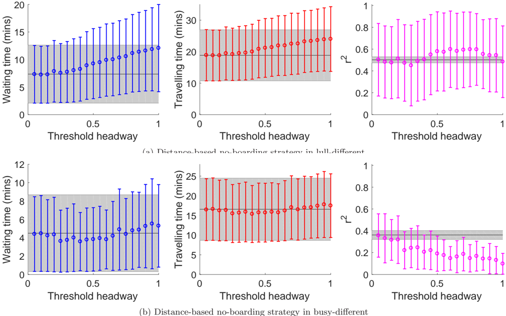
FIG. 13 Results of the no-boarding strategy in the two different-velocity scenarios. Each colored point represents the mean and standard deviation of the measured quantities calculated from 100 realizations of each parameter value. The black line and grey shaded area of each graph denote the mean and standard deviation of the measured quantities from a control case, which are simulation runs of the same parameter values, without any intervention strategies.
FIG. 13 Results of the no-boarding strategy in the two different-velocity scenarios. Each colored point represents the mean and standard deviation of the measured quantities calculated from 100 realizations of each parameter value. The black line and grey shaded area of each graph denote the mean and standard deviation of the measured quantities from a control case, which are simulation runs of the same parameter values, without any intervention strategies.CC-BY · From the PDF
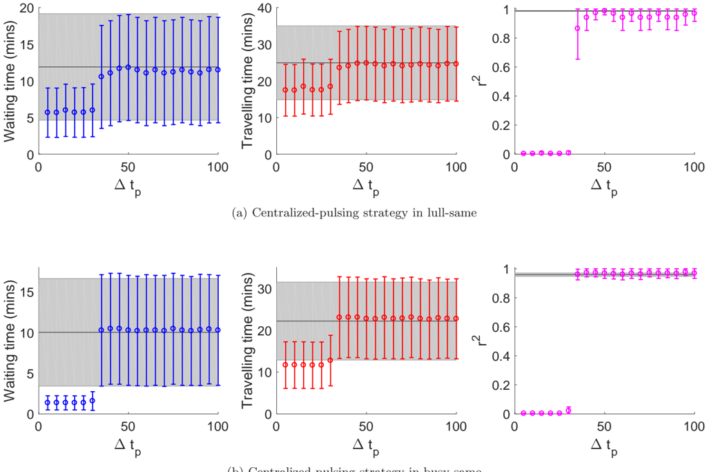
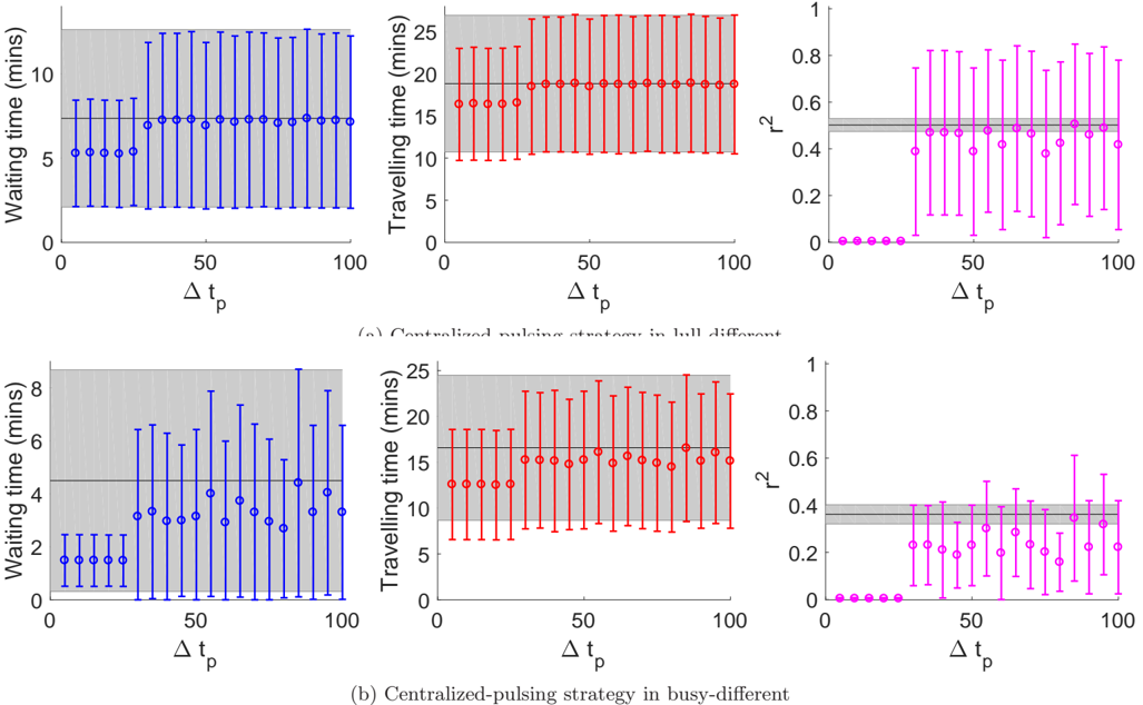
FIG. 14 Results of the centralized-pulsing strategy in the two different-velocity scenarios. Each colored point represents the mean and standard deviation of the measured quantities calculated from 100 realizations of each parameter value. The black line and grey shaded area of each graph denote the mean and standard deviation of the measured quantities from a control case, which are simulation runs of the same parameter values, without any intervention strategies.
FIG. 14 Results of the centralized-pulsing strategy in the two different-velocity scenarios. Each colored point represents the mean and standard deviation of the measured quantities calculated from 100 realizations of each parameter value. The black line and grey shaded area of each graph denote the mean and standard deviation of the measured quantities from a control case, which are simulation runs of the same parameter values, without any intervention strategies.CC-BY · From the PDF
FIG. 15 Scatter plot of all ˜ x i,t +1 , with a fitted line representing the average route taken by the buses.
FIG. 15 Scatter plot of all ˜ x i,t +1 , with a fitted line representing the average route taken by the buses.CC-BY · From the PDF
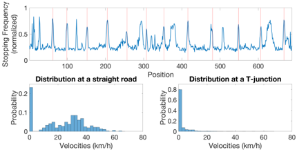
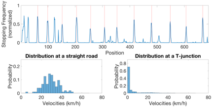
FIG. 16 Graphs of normalized stopping frequency i.e. probability of bus stopping at a each position along the bus route, and velocity distributions of two different positions on the road. These graph are derived from the raw data collected over 13 weeks. Red lines on the graph are the sites where there are bus stops.
FIG. 16 Graphs of normalized stopping frequency i.e. probability of bus stopping at a each position along the bus route, and velocity distributions of two different positions on the road. These graph are derived from the raw data collected over 13 weeks. Red lines on the graph are the sites where there are bus stops.CC-BY · From the PDF
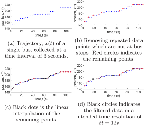
FIG. 17 Illustration of the interpolation process done to filter out false occurrence of zero velocities.
FIG. 17 Illustration of the interpolation process done to filter out false occurrence of zero velocities.CC-BY · From the PDF
FIG. 18 Graphs of normalized stopping frequency along the bus route, and velocity distributions of two different positions on the road. These graph are derived after the filtering process as described. Red lines on the graph are the sites where there are bus stops.
FIG. 18 Graphs of normalized stopping frequency along the bus route, and velocity distributions of two different positions on the road. These graph are derived after the filtering process as described. Red lines on the graph are the sites where there are bus stops.CC-BY · From the PDF

Verification

Claims the paper makes

The claims and statistics of this paper haven’t been checked yet.

Run the check — free, no account needed. It reads the open-access text and checks the sources it cites.

A few free checks a day · papers already verified open instantly · results are public

Claims other papers make about this one

Each is checked against this paper’s own text: does it say what the citing paper says it does?

Self-check

Percentages, sums and reported differences re-computed from the paper’s own numbers.

The self-check needs the paper’s full text.

Citations

Cites

Show all 1 references

Research works printed but not linked: 51

  1. NewellG. F.andPottsR. B. Maintaining a bus schedule Proceedings of the 2nd Australian Road Research Board (ARRB) Conference 1964 Melbourne Australia 388–393.
  2. 10.1371/journal.pone.0007292 · DOI
  3. 10.1007/s12469-016-0126-y · DOI · Paper page
  4. 10.1038/s41598-019-43310-7 · DOI
  5. ChewL. Y. SawV.-L. andPangY. E. I. Stability of anti-bunched buses and local unidirectional kuramoto oscillators Proceedings of the 15th International Conference on Dynamical Systems—Theory and Application December 2019 Łódż Poland.
  6. 10.1287/trsc.6.1.52 · DOI
  7. 10.1287/trsc.8.3.248 · DOI
  8. 10.1002/atr.5670200106 · DOI
  9. 10.1108/9780585474182-007 · DOI
  10. 10.1007/978-3-642-85970-0_16 · DOI
  11. 10.1016/j.ijtm.2005.02.001 · DOI
  12. 10.1080/15472450590934642 · DOI
  13. 10.1016/j.trb.2009.04.002 · DOI · Paper page
  14. 10.1007/s10489-007-0112-9 · DOI
  15. 10.1016/j.trb.2010.06.005 · DOI
  16. 10.1109/tits.2012.2188394 · DOI
  17. 10.1016/j.trc.2013.06.004 · DOI
  18. 10.1016/j.tra.2014.09.007 · DOI
  19. 10.1016/j.trb.2017.06.019 · DOI
  20. 10.1155/2018/9407801 · DOI
  21. 10.1016/j.trb.2018.06.001 · DOI
  22. 10.1155/2019/2452348 · DOI
  23. 10.1016/j.tre.2019.08.012 · DOI
  24. 10.1016/j.trb.2019.01.010 · DOI
  25. 10.1016/j.trc.2017.07.012 · DOI
  26. 10.1016/j.tra.2008.01.018 · DOI
  27. 10.1073/pnas.1016507108 · DOI · Paper page
  28. 10.1371/journal.pone.0109966 · DOI
  29. 10.1007/978-3-319-93372-6_31 · DOI
  30. 10.1016/j.trc.2011.01.003 · DOI
  31. LiuR.andSinhaS. Modelling urban bus service and passenger reliability Proceedings of the The Third International Symposium on Transportation Network Reliability July 2007 The Hague Netherlands.
  32. 10.1080/03081060802086512 · DOI
  33. 10.1016/j.trc.2013.12.005 · DOI
  34. 10.1016/j.trb.2016.07.005 · DOI
  35. 10.1088/0143-0807/29/1/015 · DOI
  36. 10.1016/j.trb.2013.01.008 · DOI
  37. 10.1016/j.trb.2009.04.003 · DOI
  38. 10.1155/2018/9714046 · DOI
  39. 10.1371/journal.pone.0230377 · DOI
  40. 10.1017/CBO9780511755743 · DOI
  41. 10.1109/tits.2016.2542268 · DOI
  42. 10.1155/2020/7274254 · DOI
  43. Binder K., 1975, Dynamics of First Order Phase Transitions
  44. 10.1017/CBO9780511564284 · DOI
  45. 10.1016/S1062-7901(06)80014-5 · DOI
  46. 10.1016/s0378-4371(02)01036-1 · DOI
  47. 10.1007/978-3-662-10583-2_10 · DOI
  48. 10.1088/2632-072x/ab4af5 · DOI
  49. 10.1051/jp1:1992277 · DOI
  50. 10.1088/1674-1056/17/5/053 · DOI
  51. 10.1103/physreve.90.032810 · DOI

Cited by

Metadata

Authors
Quek, W. L., Chung, N. N., Saw, V.-L., & Chew, L. Y.
Venue
Complexity
Publisher
Wiley
Published
2021-01
Volume
2021
Issue
1
ISSN
  • 1076-2787
  • 1099-0526
Cited by
10
References
1
Language
en
Funders
  • Joint WASP/NTU Programme (M4082189, M4082418)
  • DSAIR@NTU (M4082189, M4082418)

About these checks

Registry, retraction, Cites and statistics results are computed, not judged, with one exception: a printed reference that no index lists is read once by a model before it counts as a citation error. Claims are extracted by a model and kept only when their quote appears verbatim in the text; each cited source is then checked, with a model’s help, for whether it says what the claim relies on. Those verdicts can be wrong — read the claim’s quote and the cited source before relying on one.

Statistics and arithmetic are recomputed, not judged.

Confidence bands are shown only for fields calibrated on our annotated test set. None is calibrated yet, so no band is shown.

What counts as a claim ›How we measure confidence ›How we check this ›

Are you an author, or do you see a problem with this page? Request a review

Data sources

Bibliographic data: Semantic Scholar, OpenAlex, Crossref.

Contains information from the Semantic Scholar Academic Graph Datasets, made available under the ODC Attribution License (ODC-BY 1.0).

Semantic Scholar’s data is described in: Kinney, R., et al. (2023). The Semantic Scholar Open Data Platform. arXiv:2301.10140.