

The DOI matches its Crossref record; 41 of the 42 references it cites were found in a registry or an index.
Network motifs: Structure does not determine function.
Open accessAbstract
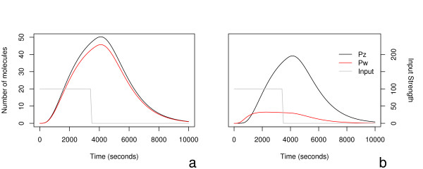
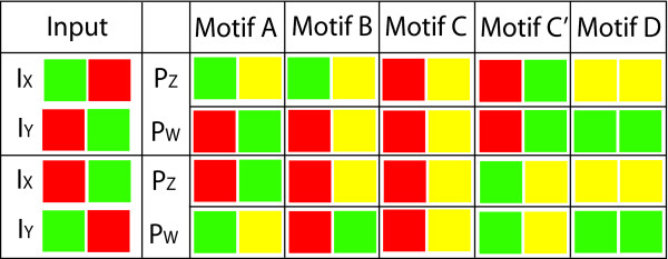
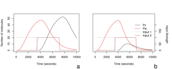
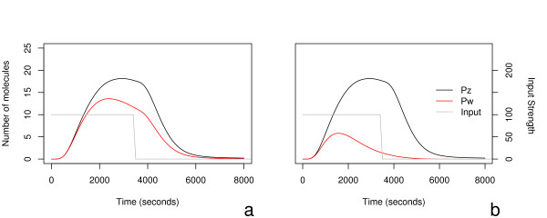
Background: A number of publications have recently examined the occurrence and properties of the feed-forward motif in a variety of networks, including those that are of interest in genome biology, such as gene networks. The present work looks in some detail at the dynamics of the bi-fan motif, using systems of ordinary differential equations to model the populations of transcription factors, mRNA and protein, with the aim of extending our understanding of what appear to be important building blocks of gene network structure. Results: We develop an ordinary differential equation model of the bi-fan motif and analyse variants of the motif corresponding to its behaviour under various conditions. In particular, we examine the effects of different steady and pulsed inputs to five variants of the bifan motif, based on evidence in the literature of bifan motifs found in Saccharomyces cerevisiae (commonly known as baker's yeast). Using this model, we characterize the dynamical behaviour of the bi-fan motif for a wide range of biologically plausible parameters and configurations. We find that there is no characteristic behaviour for the motif, and with the correct choice of parameters and of internal structure, very different, indeed even opposite behaviours may be obtained. Conclusion: Even with this relatively simple model, the bi-fan motif can exhibit a wide range of dynamical responses. This suggests that it is difficult to gain significant insights into biological function simply by considering the connection architecture of a gene network, or its decomposition into simple structural motifs. It is necessary to supplement such structural information by kinetic parameters, or dynamic time series experimental data, both of which are currently difficult to obtain.
Overview
The claims and statistics of this paper haven’t been checked yet.
Run the check — free, no account needed. It reads the open-access text and checks the sources it cites.
Integrity signals
Registry
Cites
Statistics
Figures
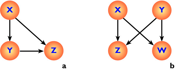
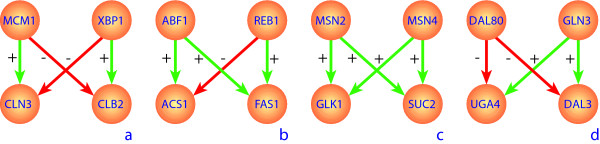
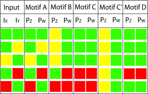
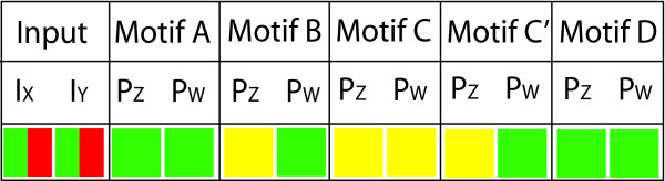
Verification
Claims the paper makes
The claims and statistics of this paper haven’t been checked yet.
Run the check — free, no account needed. It reads the open-access text and checks the sources it cites.
Claims other papers make about this one
Each is checked against this paper’s own text: does it say what the citing paper says it does?
The source backs part of the claim, not all of it — or backs it for a different population, condition or comparison.
In the citing paper
“A major challenge with such models, however, is that they often possess tens or even hundreds of free parameters whose values can significantly affect model behavior [5,6].”
From Universally Sloppy Parameter Sensitivities in Systems Biology Models (2007) · cites this paper as [5]
Experimental — accuracy not yet measured
Self-check
Percentages, sums and reported differences re-computed from the paper’s own numbers.
The self-check needs the paper’s full text.
Citations
Cites
Exact stochastic simulation of coupled chemical reactions
Gillespie, D. T. (1977) · The Journal of Physical Chemistry · doi:10.1021/j100540a008 · Cited by 10,215
Network motifs: simple building blocks of complex networks.
Milo, R., Shen-Orr, S., Itzkovitz, S., Kashtan, N., Chklovskii, D., & Alon, U. (2002) · Science · doi:10.1126/science.298.5594.824 · Cited by 7,368
Structure and function of the feed-forward loop network motif
Mangan, S., & Alon, U. (2003) · Proceedings of the National Academy of Sciences · doi:10.1073/pnas.2133841100 · Cited by 1,827
Superfamilies of Evolved and Designed Networks
Milo, R., Itzkovitz, S., Kashtan, N., Levitt, R., Shen-Orr, S. S., Ayzenshtat, I., Sheffer, M., & Alon, U. S. (2004) · Science · doi:10.1126/science.1089167 · Cited by 1,427
The Coherent Feedforward Loop Serves as a Sign-sensitive Delay Element in Transcription Networks
Mangan, S., Zaslaver, A., & Alon, U. S. (2003) · Journal of Molecular Biology · doi:10.1016/j.jmb.2003.09.049 · Cited by 548
How the λ repressor and cro work
Ptashne, M., Jeffrey, A., Johnson, A. D., Maurer, R., Meyer, B. J., Pabo, C. O., Roberts, T. M., & Sauer, R. T. (1980) · Cell · doi:10.1016/0092-8674(80)90383-9 · Cited by 452
Dynamic Properties of Network Motifs Contribute to Biological Network Organization
Prill, R. J., Iglesias, P. A., & Levchenko, A. (2005) · PLoS Biology · doi:10.1371/journal.pbio.0030343 · Cited by 378
Cosma, M. P. (2002) · Molecular Cell · doi:10.1016/s1097-2765(02)00604-4 · Cited by 266
Artzy‐Randrup, Y., Fleishman, S. J., Ben‐Tal, N., & Stone, L. (2004) · Science · doi:10.1126/science.1099334 · Cited by 254
Estruch, F., & Carlson, M. (1993) · Molecular and Cellular Biology · doi:10.1128/mcb.13.7.3872-3881.1993 · Cited by 221
Convergent evolution of gene circuits
Conant, G. C., & Wagner, A. (2003) · Nature Genetics · doi:10.1038/ng1181 · Cited by 198
Proft, M., & Serrano, R. (1999) · Molecular and Cellular Biology · doi:10.1128/mcb.19.1.537 · Cited by 180
Vincent, O., & Carlson, M. (1998) · The EMBO Journal · doi:10.1093/emboj/17.23.7002 · Cited by 128
Mcm1 Is Required To Coordinate G 2 -Specific Transcription in Saccharomyces cerevisiae
Althöfer, H., Schleiffer, A., Wassmann, K., Nordheim, A., & Ammerer, G. (1995) · Molecular and Cellular Biology · doi:10.1128/mcb.15.11.5917 · Cited by 127
Back to the biology in systems biology: What can we learn from biomolecular networks?
Huang, S. (2004) · Briefings in Functional Genomics and Proteomics · doi:10.1093/bfgp/2.4.279 · Cited by 125
Coffman, J. A., Rai, R., Loprete, D. M., Cunningham, T. S., Svetlov, V. V., & Cooper, T. (1997) · Journal of Bacteriology · doi:10.1128/jb.179.11.3416-3429.1997 · Cited by 118
Nehlin, J. O., Carlberg, M., & Ronne, H. (1992) · Nucleic Acids Research · doi:10.1093/nar/20.20.5271 · Cited by 115
Hiroi, H., Christenson, L. K., Chang, L., Sammel, M. D., Berger, S. L., & Strauss, J. F. (2004) · Molecular Endocrinology · doi:10.1210/me.2003-0305 · Cited by 103
Brindle, P. K., Holland, J. P., Willett, C., Innis, M. A., & Holland, M. J. (1990) · Molecular and Cellular Biology · doi:10.1128/mcb.10.9.4872-4885.1990 · Cited by 100
Huie, M. A., Scott, E. W., Drazinic, C. M., López, M. C., Hornstra, I. K., Yang, T. P., & Baker, H. V. (1992) · Molecular and Cellular Biology · doi:10.1128/mcb.12.6.2690 · Cited by 98
The Role of Dimerization in Noise Reduction of Simple Genetic Networks
Bundschuh, R. A., Hayot, F., & Jayaprakash, C. (2002) · Journal of Theoretical Biology · doi:10.1006/jtbi.2003.3164 · Cited by 97
Schöler, A., & Schüller, H. (1994) · Molecular and Cellular Biology · doi:10.1128/mcb.14.6.3613 · Cited by 85
Kratzer, S., & Schüller, H. (1997) · Molecular Microbiology · doi:10.1046/j.1365-2958.1997.5611937.x · Cited by 80
Cunningham, T. S., & Cooper, T. (1993) · Journal of Bacteriology · doi:10.1128/jb.175.18.5851-5861.1993 · Cited by 72
Murén, E., Öyen, M., Barmark, G., & Ronne, H. (2000) · Yeast · doi:10.1002/1097-0061(20010130)18:2 · Cited by 64
Kratzer, S., & Schüller, H. (1995) · Gene · doi:10.1016/0378-1119(95)00289-i · Cited by 61
Talibi, D., Grenson, M., & André, B. (1995) · Nucleic Acids Research · doi:10.1093/nar/23.4.550 · Cited by 59
Bu, Y. (1998) · Nucleic Acids Research · doi:10.1093/nar/26.4.1002 · Cited by 55
Cunningham, T. S., Svetlov, V. V., Rai, R., Smart, W. C., & Cooper, T. (1996) · Journal of Bacteriology · doi:10.1128/jb.178.12.3470-3479.1996 · Cited by 55
CLN1 and Its Repression by Xbp1 Are Important for Efficient Sporulation in Budding Yeast
Mai, B., & Breeden, L. L. (2000) · Molecular and Cellular Biology · doi:10.1128/mcb.20.2.478-487.2000 · Cited by 49
André, B., Talibi, D., Soussi‐Boudekou, S., Hein, C., VISSERS, S., & Coornaert, D. (1995) · Nucleic Acids Research · doi:10.1093/nar/23.4.558 · Cited by 48
Schüller, H., Schütz, A., Knab, S., Hoffmann, B., & Schweizer, E. (1994) · European Journal of Biochemistry · doi:10.1111/j.1432-1033.1994.00213.x · Cited by 45
p53 Targets Chromatin Structure Alteration to Repress α-Fetoprotein Gene Expression
Ogden, S. K., Lee, K. C., Wernke-Dollries, K., Stratton, S. A., Aronow, B. J., & Barton, M. C. (2001) · Journal of Biological Chemistry · doi:10.1074/jbc.c100381200 · Cited by 43
Willett, C., Gelfman, C. M., & Holland, M. J. (1993) · Molecular and Cellular Biology · doi:10.1128/mcb.13.4.2623 · Cited by 32
A feedforward loop motif in transcriptional regulation: induction and repression
Hayot, F., & Jayaprakash, C. (2005) · Journal of Theoretical Biology · doi:10.1016/j.jtbi.2004.11.010 · Cited by 31
Moreno‐Herrero, F., Herrero, P., Colchero, J., Baró, A. M., & Moreno, F. (1999) · FEBS Letters · doi:10.1016/s0014-5793(99)01289-2 · Cited by 31
Holland, J. P., Brindle, P. K., & Holland, M. J. (1990) · Molecular and Cellular Biology · doi:10.1128/mcb.10.9.4863 · Cited by 28
Machida, M., Uemura, H., Jigami, Y., & Tanaka, H. (1988) · Nucleic Acids Research · doi:10.1093/nar/16.4.1407 · Cited by 27
Herrero, P., FLORES, L., Tamara de la, C. E. R. A., & MORENO, F. (1999) · Biochemical Journal · doi:10.1042/0264-6021:3430319 · Cited by 25
Zaragoza, Ó., Vincent, O., & Gancedo, J. M. (2001) · Biochemical Journal · doi:10.1042/0264-6021:3590193 · Cited by 23
Machida, M., Jigami, Y., & Tanaka, H. (1989) · European Journal of Biochemistry · doi:10.1111/j.1432-1033.1989.tb15020.x · Cited by 13
Cited by
Sorted by citations
Network motifs: theory and experimental approaches
Alon, U. (2007) · Nature Reviews Genetics · doi:10.1038/nrg2102 · Cited by 3,279
Modelling and analysis of gene regulatory networks
Karlebach, G., & Shamir, R. (2008) · Nature Reviews Molecular Cell Biology · doi:10.1038/nrm2503 · Cited by 1,296
Universally Sloppy Parameter Sensitivities in Systems Biology Models
Gutenkunst, R. N., Waterfall, J. J., Casey, F. P., Brown, K. S., Myers, C. R., & Sethna, J. P. (2007) · PLoS Computational Biology · doi:10.1371/journal.pcbi.0030189 · Cited by 1,261
“A major challenge with such models, however, is that they often possess tens or even hundreds of free parameters whose values can significantly affect model behavior [5, 6].”
BackgroundUsing graph theory to analyze biological networks
Pavlopoulos, G. A., Secrier, M., Moschopoulos, C. N., Soldatos, T. G., Κοσσίδα, Σ., Aerts, J. A., Schneider, R., & Bagos, P. G. (2011) · BioData Mining · doi:10.1186/1756-0381-4-10 · Cited by 821
Gene Regulatory Network Inference from Single-Cell Data Using Multivariate Information Measures
Chan, T. E., Stumpf, M. P. H., & Babtie, A. C. (2017) · Cell Systems · doi:10.1016/j.cels.2017.08.014 · Cited by 578
Self-citation
Metadata
- Authors
- Ingram, P. J., Stumpf, M. P., & Stark, J.
- Affiliations
- Imperial College London (GB)
- Corresponding author
- Ingram, Piers J
- ORCID
- Stumpf, Michael PH
- Venue
- BMC Genomics
- Published
- 2006-05-05
- Volume
- 7
- Issue
- 1
- Pages
- 108-108
- ISSN
- 1471-2164 (ISSN-L)
- PMC
- PMC1488845
- OpenAlex
- W1808967201
- Cited by
- 267
- References
- 42
- Citations by year
- 2026: 13 · 2025: 5 · 2024: 8 · 2023: 5 · 2022: 4 · 2021: 13 · 2020: 10 · 2019: 11 · 2018: 16 · 2017: 9 · 2016: 20 · 2015: 12 · 2014: 19 · 2013: 29 · 2012: 15
- FWCI
- 6.53
- Type
- journal article
- Language
- en
- Open access
- gold
- doi.org
- Licence
- Locations
- BMC Genomics (publishedVersion, cc-by)
- PubMed Central (publishedVersion, cc-by)
- PubMed (publishedVersion)
- DOAJ (DOAJ: Directory of Open Access Journals) (submittedVersion, cc-by-sa)
- Minerva Access (University of Melbourne) (submittedVersion, cc-by)
- Funders
- Wellcome Trust
- Topics
- Life Sciences › Biochemistry, Genetics and Molecular Biology › Molecular Biology › Gene Regulatory Network Analysis
- Life Sciences › Biochemistry, Genetics and Molecular Biology › Molecular Biology › Bioinformatics and Genomic Networks
- Life Sciences › Biochemistry, Genetics and Molecular Biology › Molecular Biology › Microbial Metabolic Engineering and Bioproduction
- Keywords
- network motifs, gene regulatory networks, transcription factors, ordinary differential equation model, network dynamics, Saccharomyces cerevisiae, kinetic parameters, structure-function relationship
- MeSH terms
- Genes, Fungal, Models, Biological, Saccharomyces cerevisiae, Transcription, Genetic, Gene Expression Regulation, Fungal, Computational Biology, Amino Acid Motifs
About these checks
Registry, retraction, Cites and statistics results are computed, not judged, with one exception: a printed reference that no index lists is read once by a model before it counts as a citation error. Claims are extracted by a model and kept only when their quote appears verbatim in the text; each cited source is then checked, with a model’s help, for whether it says what the claim relies on. Those verdicts can be wrong — read the claim’s quote and the cited source before relying on one.
Statistics and arithmetic are recomputed, not judged.
Confidence bands are shown only for fields calibrated on our annotated test set. None is calibrated yet, so no band is shown.
What counts as a claim ›How we measure confidence ›How we check this ›
Are you an author, or do you see a problem with this page? Request a review
