

The DOI matches its Crossref record; 50 of the 50 references it cites were found in a registry or an index.
Probability Matching as a Computational Strategy Used in Perception
Open accessAbstract
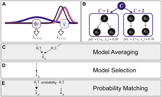
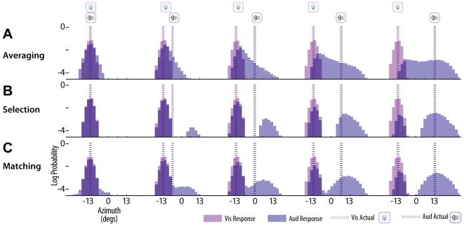
The question of which strategy is employed in human decision making has been studied extensively in the context of cognitive tasks; however, this question has not been investigated systematically in the context of perceptual tasks. The goal of this study was to gain insight into the decision-making strategy used by human observers in a low-level perceptual task. Data from more than 100 individuals who participated in an auditory-visual spatial localization task was evaluated to examine which of three plausible strategies could account for each observer's behavior the best. This task is very suitable for exploring this question because it involves an implicit inference about whether the auditory and visual stimuli were caused by the same object or independent objects, and provides different strategies of how using the inference about causes can lead to distinctly different spatial estimates and response patterns. For example, employing the commonly used cost function of minimizing the mean squared error of spatial estimates would result in a weighted averaging of estimates corresponding to different causal structures. A strategy that would minimize the error in the inferred causal structure would result in the selection of the most likely causal structure and sticking with it in the subsequent inference of location-"model selection." A third strategy is one that selects a causal structure in proportion to its probability, thus attempting to match the probability of the inferred causal structure. This type of probability matching strategy has been reported to be used by participants predominantly in cognitive tasks. Comparing these three strategies, the behavior of the vast majority of observers in this perceptual task was most consistent with probability matching. While this appears to be a suboptimal strategy and hence a surprising choice for the perceptual system to adopt, we discuss potential advantages of such a strategy for perception.
Overview
The claims and statistics of this paper haven’t been checked yet.
Run the check — free, no account needed. It reads the open-access text and checks the sources it cites.
Integrity signals
Registry
Cites
Statistics
Figures
Verification
Claims the paper makes
The claims and statistics of this paper haven’t been checked yet.
Run the check — free, no account needed. It reads the open-access text and checks the sources it cites.
Claims other papers make about this one
Each is checked against this paper’s own text: does it say what the citing paper says it does?
In the citing paper
“Bayesian samplers can match behavioral stochasticity in tasks such as perception, categorization, causal reasoning, and decision making [20,21,23,24].”
From Bayesian Brains without Probabilities (2016) · cites this paper as [23]
Self-check
Percentages, sums and reported differences re-computed from the paper’s own numbers.
The self-check needs the paper’s full text.
Citations
Cites
Theory of games and economic behavior
Garcia, S. R., & Miller, S. J. (2019) · American Mathematical Society eBooks · doi:10.1090/mbk/121/32 · Cited by 16,777
(1966) · Medical Entomology and Zoology · Cited by 10,293
Signal detection theory and psychophysics
Ingleby, D. (1967) · Journal of Sound and Vibration · doi:10.1016/0022-460x(67)90197-6 · Cited by 8,616
Jeffreys, H., Moran, P. A. P., & Chatfield, C. (1922) · Nature · doi:10.1038/109132a0 · Cited by 7,877
A note on a general definition of the coefficient of determination
NAGELKERKE, N. J. D. (1991) · Biometrika · doi:10.1093/biomet/78.3.691 · Cited by 5,927
The Theory of Games and Economic Behavior
Harrison, R. W., von Neumann, J., & Morgenstern, O. (1945) · Journal of Farm Economics · doi:10.2307/1232672 · Cited by 5,318
Humans integrate visual and haptic information in a statistically optimal fashion
Ernst, M. O., & Banks, M. S. (2002) · Nature · doi:10.1038/415429a · Cited by 4,844
Individual differences in reasoning: Implications for the rationality debate?
Stanovich, K. E., & West, R. F. (2000) · Behavioral and Brain Sciences · doi:10.1017/s0140525x00003435 · Cited by 4,481
The Ventriloquist Effect Results from Near-Optimal Bimodal Integration
Alais, D., & Burr, D. (2004) · Current Biology · doi:10.1016/j.cub.2004.01.029 · Cited by 1,936
Perception as Bayesian Inference
(1996) · doi:10.1017/cbo9780511984037 · Cited by 1,425
Cited by
Sorted by citations
Behavioral, Neural, and Computational Principles of Bodily Self-Consciousness
Blanke, O., Slater, M., & Serino, A. (2015) · Neuron · doi:10.1016/j.neuron.2015.09.029 · Cited by 698
Kilteni, K., Maselli, A., Kording, K. P., & Slater, M. (2015) · Frontiers in Human Neuroscience · doi:10.3389/fnhum.2015.00141 · Cited by 549
Bayesian just-so stories in psychology and neuroscience.
Bowers, J. S., & Davis, C. J. (2012) · Psychological Bulletin · doi:10.1037/a0026450 · Cited by 436
Cortical Hierarchies Perform Bayesian Causal Inference in Multisensory Perception
Rohe, T., & Noppeney, U. (2015) · PLOS Biology · doi:10.1371/journal.pbio.1002073 · Cited by 344
Bayesian Brains without Probabilities
Sanborn, A. N., & Chater, N. (2016) · Trends in Cognitive Sciences · doi:10.1016/j.tics.2016.10.003 · Cited by 307
Metadata
- Authors
- Wozny, D. R., Beierholm, U. R., & Shams, L.
- Affiliations
- University of California, Los Angeles (US)
- Gatsby Computational Neuroscience Unit (GB)
- Corresponding author
- Shams, Ladan
- Venue
- PLoS Computational Biology
- Publisher
- Public Library of Science (PLoS)
- Published
- 2010-08-05
- Volume
- 6
- Issue
- 8
- Pages
- e1000871
- ISSN
- 1553-734X (ISSN-L)
- 1553-7358
- PMC
- PMC2916852
- OpenAlex
- W2067064274
- Cited by
- 265
- References
- 50
- Citations by year
- 2026: 14 · 2025: 18 · 2024: 48 · 2023: 15 · 2022: 15 · 2021: 21 · 2020: 15 · 2019: 20 · 2018: 24 · 2017: 18 · 2016: 16 · 2015: 15 · 2014: 5 · 2013: 4 · 2012: 7
- FWCI
- 8.74
- Type
- journal article
- Language
- en
- Open access
- gold
- doi.org
- Locations
- PLoS Computational Biology (publishedVersion, cc-by)
- PubMed Central (publishedVersion, cc-by)
- PubMed (publishedVersion)
- RePEc: Research Papers in Economics (submittedVersion)
- DOAJ (DOAJ: Directory of Open Access Journals) (submittedVersion, cc-by-sa)
- UCL Discovery (University College London) (submittedVersion)
- eScholarship (California Digital Library) (submittedVersion)
- eScholarship (California Digital Library) (submittedVersion, cc-by)
- Max Planck Digital Library (submittedVersion, other-oa)
- Figshare (submittedVersion, cc-by)
- Durham Research Online (Durham University) (submittedVersion, cc-by)
- University of Birmingham Research Portal (University of Birmingham) (submittedVersion, other-oa)
- MPG.PuRe (Max Planck Society) (submittedVersion, other-oa)
- Funders
- National Institutes of Health
- Topics
- Social Sciences › Psychology › Experimental and Cognitive Psychology › Multisensory perception and integration
- Life Sciences › Neuroscience › Cognitive Neuroscience › Visual perception and processing mechanisms
- Physical Sciences › Computer Science › Artificial Intelligence › Bayesian Modeling and Causal Inference
- Keywords
- probability matching, perceptual decision making, causal inference, model selection, weighted averaging, suboptimal strategies, cross-modal integration, perceptual inference
- MeSH terms
- Decision Making, Female, Humans, Male, Probability Learning, Sound Localization, Visual Perception, Young Adult
About these checks
Registry, retraction, Cites and statistics results are computed, not judged, with one exception: a printed reference that no index lists is read once by a model before it counts as a citation error. Claims are extracted by a model and kept only when their quote appears verbatim in the text; each cited source is then checked, with a model’s help, for whether it says what the claim relies on. Those verdicts can be wrong — read the claim’s quote and the cited source before relying on one.
Statistics and arithmetic are recomputed, not judged.
Confidence bands are shown only for fields calibrated on our annotated test set. None is calibrated yet, so no band is shown.
What counts as a claim ›How we measure confidence ›How we check this ›
Are you an author, or do you see a problem with this page? Request a review
