

The DOI matches its Crossref record; 69 of the 70 references it cites were found in a registry or an index; none of the 29 sources its claims cite is checked for support yet.
Bonsai Trees in Your Head: How the Pavlovian System Sculpts Goal-Directed Choices by Pruning Decision Trees
Open accessAbstract
When planning a series of actions, it is usually infeasible to consider all potential future sequences; instead, one must prune the decision tree. Provably optimal pruning is, however, still computationally ruinous and the specific approximations humans employ remain unknown. We designed a new sequential reinforcement-based task and showed that human subjects adopted a simple pruning strategy: during mental evaluation of a sequence of choices, they curtailed any further evaluation of a sequence as soon as they encountered a large loss. This pruning strategy was Pavlovian: it was reflexively evoked by large losses and persisted even when overwhelmingly counterproductive. It was also evident above and beyond loss aversion. We found that the tendency towards Pavlovian pruning was selectively predicted by the degree to which subjects exhibited sub-clinical mood disturbance, in accordance with theories that ascribe Pavlovian behavioural inhibition, via serotonin, a role in mood disorders. We conclude that Pavlovian behavioural inhibition shapes highly flexible, goal-directed choices in a manner that may be important for theories of decision-making in mood disorders.
Overview
AI snapshot
Written from the paper’s full text.
TL;DR
Humans planning sequences prune decision trees by curtailing evaluation after large losses, a Pavlovian response that persists even when counterproductive. Computational modeling shows this specific pruning is distinct from general discounting and loss aversion, and correlates with subclinical depressive symptoms.
Key findings
- Subjects adopted a simple pruning strategy: they stopped evaluating a sequence when they encountered a large loss, even when this was costly. In group −140 pruning was never disadvantageous, but in groups −70 and −100 it was increasingly counterproductive, yet subjects continued to prune.
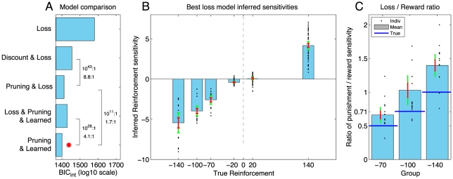
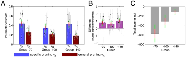
- The most parsimonious model was “Pruning & Learned,” which separated general pruning from specific pruning after large punishments. Specific pruning exceeded general pruning in 14/15, 12/16, and 14/15 subjects in the −70, −100, and −140 groups, respectively. This model correctly predicted 91% of choices; the full look-ahead model predicted 77% of choices and had a mean predictive probability of 0.71.
- Pruning was evident above and beyond loss aversion. Subjects were approximately 1.4 times more sensitive to punishments than to equal-sized rewards, but adding loss aversion to the best model did not improve parsimony.
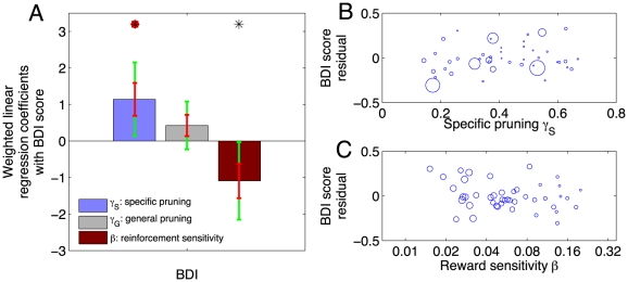
- BDI score positively correlated with the specific pruning parameter, but not with general pruning. A negative correlation between BDI and reward sensitivity did not survive correction for multiple comparisons. NEO agreeableness positively correlated with the Learned Pavlovian influence and survived full correction for 60 comparisons; no significant correlation with NEO neuroticism was found.
Methods
- Forty-six volunteers (23 female, mean age 23.84 years) were recruited and screened; groups received different large losses: −70 (n=15), −100 (n=16), and −140 (n=15). Subjects learned a deterministic six-state transition matrix, then completed two blocks of 24 choice episodes with sequence lengths of 2–8; the first block was discarded and the second analyzed. On half the trials, subjects planned their last 2–4 moves together without intermittent feedback.
- Computational models included full look-ahead, discounting, pruning (general and specific), learned Pavlovian attraction/repulsion, loss aversion, and a habitual SARSA model. Models were fit with Bayesian model fitting and compared using integrated Bayesian Information Criterion at the group level.
- Psychometric correlates were assessed with a weighted hierarchical multivariate regression, orthogonalizing age, sex, IQ, Digit Span, NEO measures, STAI, and BDI.
Limitations
- The paper states that the sample was healthy volunteers with only very mild depressive symptoms, so the BDI correlation cannot be taken as direct evidence that mildly raised BDI scores measure vulnerability to depression; predictions about clinical depression and serotonin depletion remain to be tested. It also states that no significant correlation with NEO neuroticism was found.
- The paper notes that in group −140 there was always an optimal sequence avoiding the large loss, making that group’s behavioral statistic difficult to interpret; at depths of 6 or more, the number of events was small, limiting power; and some missing age/STAI data excluded subjects from psychometric analyses.
- Evident from the text: the task uses a fixed deterministic transition matrix and specific reinforcement structure, and the conclusions depend on the fitted model space; model comparison did not support separate group differences in pruning despite apparent behavioral differences.
Model-written summary. Check it against the paper before relying on it.
Integrity signals
Registry
Cites
Statistics
Figures
Verification
Claims the paper makes
35 Own result · 20 Not checked yet · 9 Own interpretation · 6 Own method · 4 No basis given
A result the paper reports from its own data — it cites no other source for it, so there is none to check. The quote shows it is in the paper.
In the paper
“Again, we applied Bayesian model comparison and found strong evidence for such a separation (Figure 4C).”
§ Bonsai Trees in Your Head: How the Pavlovian System Sculpts Goal-Directed Choices by Pruning Decision Trees > Results > Decision making structure
boosted- Asserted: passes — The authors put it forward as true.
- Checkable: passes — It can be checked against evidence.
- Load-bearing: passes — The paper’s conclusions depend on it.
- Based: passes — The paper gives a reason why it holds.
A result the paper reports from its own data — it cites no other source for it, so there is none to check. The quote shows it is in the paper.
In the paper
“We found that BDI was positively correlated with the specific pruning parameter ().”
§ Bonsai Trees in Your Head: How the Pavlovian System Sculpts Goal-Directed Choices by Pruning Decision Trees > Results > Psychometric correlates
plaincorrelational- Asserted: passes — The authors put it forward as true.
- Checkable: passes — It can be checked against evidence.
- Load-bearing: passes — The paper’s conclusions depend on it.
- Based: passes — The paper gives a reason why it holds.
- Rests on an assumption: The BDI validly measures sub-clinical depressive symptoms/mood disturbance.
A result the paper reports from its own data — it cites no other source for it, so there is none to check. The quote shows it is in the paper.
In the paper
“Furthermore, this effect was specific in that there was no such correlation with general pruning .”
§ Bonsai Trees in Your Head: How the Pavlovian System Sculpts Goal-Directed Choices by Pruning Decision Trees > Results > Psychometric correlates
plaincorrelational- Asserted: passes — The authors put it forward as true.
- Checkable: passes — It can be checked against evidence.
- Load-bearing: passes — The paper’s conclusions depend on it.
- Based: passes — The paper gives a reason why it holds.
- Rests on an assumption: The BDI validly measures sub-clinical depressive symptoms/mood disturbance.
A result the paper reports from its own data — it cites no other source for it, so there is none to check. The quote shows it is in the paper.
In the paper
“Subjects were significantly seduced by the effect of these past rewards (or repulsed by punishments), again in a way that was counterproductive to optimal control.”
§ Bonsai Trees in Your Head: How the Pavlovian System Sculpts Goal-Directed Choices by Pruning Decision Trees > Discussion
plaindirect- Asserted: passes — The authors put it forward as true.
- Checkable: passes — It can be checked against evidence.
- Load-bearing: passes — The paper’s conclusions depend on it.
- Based: passes — The paper gives a reason why it holds.
A result the paper reports from its own data — it cites no other source for it, so there is none to check. The quote shows it is in the paper.
In the paper
“Subjects were worse at choosing optimal sequences when the depth was greater.”
§ Bonsai Trees in Your Head: How the Pavlovian System Sculpts Goal-Directed Choices by Pruning Decision Trees > Results
plaincorrelational- Asserted: passes — The authors put it forward as true.
- Checkable: passes — It can be checked against evidence.
- Load-bearing: passes — The paper’s conclusions depend on it.
- Based: passes — The paper gives a reason why it holds.
A result the paper reports from its own data — it cites no other source for it, so there is none to check. The quote shows it is in the paper.
In the paper
“We designed a new sequential reinforcement-based task and showed that human subjects adopted a simple pruning strategy: during mental evaluation of a sequence of choices, they curtailed any further evaluation of a sequence as soon as they encountered a large loss.”
§ Bonsai Trees in Your Head: How the Pavlovian System Sculpts Goal-Directed Choices by Pruning Decision Trees > Abstract
plaindirect- Asserted: passes — The authors put it forward as true.
- Checkable: passes — It can be checked against evidence.
- Load-bearing: passes — The paper’s conclusions depend on it.
- Based: passes — The paper gives a reason why it holds.
A result the paper reports from its own data — it cites no other source for it, so there is none to check. The quote shows it is in the paper.
In the paper
“subjects also showed a substantial increase in their propensity to prune in the face of a large negative outcome (parameter in the model).”
§ Bonsai Trees in Your Head: How the Pavlovian System Sculpts Goal-Directed Choices by Pruning Decision Trees > Discussion
plaindirect- Asserted: passes — The authors put it forward as true.
- Checkable: passes — It can be checked against evidence.
- Load-bearing: passes — The paper’s conclusions depend on it.
- Based: passes — The paper gives a reason why it holds.
- Rests on an assumption: The large losses in the task are aversive/punishing events capable of evoking Pavlovian behavioural inhibition.
A result the paper reports from its own data — it cites no other source for it, so there is none to check. The quote shows it is in the paper.
In the paper
“We found a positive correlation between NEO agreeableness and the weight of the ‘Learned Pavlovian’ influence which survived full correction for 60 comparisons .”
§ Bonsai Trees in Your Head: How the Pavlovian System Sculpts Goal-Directed Choices by Pruning Decision Trees > Results > Psychometric correlates
plaincorrelational- Asserted: passes — The authors put it forward as true.
- Checkable: passes — It can be checked against evidence.
- Load-bearing: unclear — It is unclear whether the paper’s conclusions depend on it.
- Based: passes — The paper gives a reason why it holds.
A result the paper reports from its own data — it cites no other source for it, so there is none to check. The quote shows it is in the paper.
In the paper
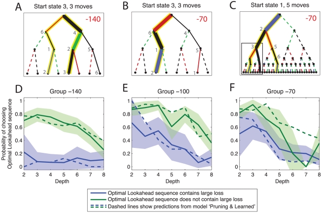
“That is, the tendency to excise subtrees lying below punishments persisted even when counterproductive in terms of outcomes.”
§ Bonsai Trees in Your Head: How the Pavlovian System Sculpts Goal-Directed Choices by Pruning Decision Trees > Introduction
plain- Asserted: passes — The authors put it forward as true.
- Checkable: passes — It can be checked against evidence.
- Load-bearing: passes — The paper’s conclusions depend on it.
- Based: passes — The paper gives a reason why it holds.
A result the paper reports from its own data — it cites no other source for it, so there is none to check. The quote shows it is in the paper.
In the paper
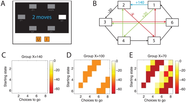
“It was striking that subjects were no less likely to prune (Figure 2C–D) even when we rendered it increasingly disadvantageous (moving from group −140 to group −70),.”
§ Bonsai Trees in Your Head: How the Pavlovian System Sculpts Goal-Directed Choices by Pruning Decision Trees > Discussion
plain- Asserted: passes — The authors put it forward as true.
- Checkable: passes — It can be checked against evidence.
- Load-bearing: passes — The paper’s conclusions depend on it.
- Based: passes — The paper gives a reason why it holds.
- It may state two separate claims as one. 24
- Probably not a substantial claim. 18
A result the paper reports from its own data — it cites no other source for it, so there is none to check. The quote shows it is in the paper.
In the paper
“Specific pruning exceeded general pruning across subjects, but there was no main effect of group and no interaction.”
§ Bonsai Trees in Your Head: How the Pavlovian System Sculpts Goal-Directed Choices by Pruning Decision Trees > Results > Pruning estimates
plainn = 15- Asserted: passes — The authors put it forward as true.
- Checkable: passes — It can be checked against evidence.
- Load-bearing: unclear — It is unclear whether the paper’s conclusions depend on it.
- Based: passes — The paper gives a reason why it holds.
It may state two separate claims as one.
A result the paper reports from its own data — it cites no other source for it, so there is none to check. The quote shows it is in the paper.
In the paper
“There was also a negative correlation between BDI score and reward sensitivity , although this did not survive correction for multiple comparisons ().”
§ Bonsai Trees in Your Head: How the Pavlovian System Sculpts Goal-Directed Choices by Pruning Decision Trees > Results > Psychometric correlates
plaincorrelational- Asserted: passes — The authors put it forward as true.
- Checkable: passes — It can be checked against evidence.
- Load-bearing: fails — The paper’s conclusions may not depend on it.
- Based: passes — The paper gives a reason why it holds.
Probably not a substantial claim. The paper’s conclusions may not depend on it. It may state two separate claims as one.
- Rests on an assumption: The BDI validly measures sub-clinical depressive symptoms/mood disturbance.
A result the paper reports from its own data — it cites no other source for it, so there is none to check. The quote shows it is in the paper.
In the paper
“Computational models which accounted for close to 90% of choices verified that the nature of pruning corresponded to the Pavlovian reflexive account in detail.”
§ Bonsai Trees in Your Head: How the Pavlovian System Sculpts Goal-Directed Choices by Pruning Decision Trees > Introduction
plaincorrelational- Asserted: passes — The authors put it forward as true.
- Checkable: passes — It can be checked against evidence.
- Load-bearing: passes — The paper’s conclusions depend on it.
- Based: passes — The paper gives a reason why it holds.
It may state two separate claims as one.
The paper states this without a source or data behind it here, so there is nothing to check it against. The quote shows it is in the paper.
In the paper
“Next, subjects could transition through losses early on in the tree, but were more reluctant to do so when they appeared deeper in the tree.”
§ Bonsai Trees in Your Head: How the Pavlovian System Sculpts Goal-Directed Choices by Pruning Decision Trees > Discussion
hedgedcorrelational- Asserted: passes — The authors put it forward as true.
- Checkable: passes — It can be checked against evidence.
- Load-bearing: passes — The paper’s conclusions depend on it.
- Based: passes — The paper gives a reason why it holds.
It may state two separate claims as one.
A result the paper reports from its own data — it cites no other source for it, so there is none to check. The quote shows it is in the paper.
In the paper
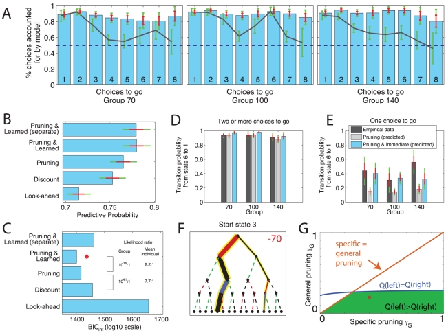
“This model ascribed the higher action value to the subjects' actual choices a total of 77% of the time (fraction of choices predicted), which is significantly better than chance (fixed effect binomial ).”
§ Bonsai Trees in Your Head: How the Pavlovian System Sculpts Goal-Directed Choices by Pruning Decision Trees > Results > Decision making structure
plaincorrelational- Asserted: passes — The authors put it forward as true.
- Checkable: passes — It can be checked against evidence.
- Load-bearing: passes — The paper’s conclusions depend on it.
- Based: passes — The paper gives a reason why it holds.
It may state two separate claims as one.
The paper states this without a source or data behind it here, so there is nothing to check it against. The quote shows it is in the paper.
In the paper
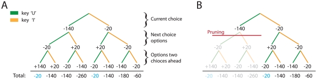
“In terms of net earnings, pruning is never advantageous (pruned values are never better than the optimal lookahead values); but pruning does not always result in losses (white areas). It is most disadvantageous in the −70 group, and it is never disadvantageous in the −140 group because there is always an equally good alternative choice sequence which avoids transitions through large losses.”
§ Bonsai Trees in Your Head: How the Pavlovian System Sculpts Goal-Directed Choices by Pruning Decision Trees > Introduction
plain- Asserted: passes — The authors put it forward as true.
- Checkable: passes — It can be checked against evidence.
- Load-bearing: passes — The paper’s conclusions depend on it.
- Based: passes — The paper gives a reason why it holds.
It may state two separate claims as one.
A result the paper reports from its own data — it cites no other source for it, so there is none to check. The quote shows it is in the paper.
In the paper
“In contrast, in the second and third experimental groups subjects incurred increasingly large costs for this pruning strategy (Figure 2D,E); yet, they continued to deploy it.”
§ Bonsai Trees in Your Head: How the Pavlovian System Sculpts Goal-Directed Choices by Pruning Decision Trees > Introduction
plaincorrelational- Asserted: passes — The authors put it forward as true.
- Checkable: passes — It can be checked against evidence.
- Load-bearing: passes — The paper’s conclusions depend on it.
- Based: passes — The paper gives a reason why it holds.
It may state two separate claims as one.
A result the paper reports from its own data — it cites no other source for it, so there is none to check. The quote shows it is in the paper.
In the paper
“This was not predicted by the pruning model: paired t-tests showed significant differences between empirical and predicted choice probabilities for each of the three groups: , ; , ; and , , for groups −70, −100 and −140 respectively.”
§ Bonsai Trees in Your Head: How the Pavlovian System Sculpts Goal-Directed Choices by Pruning Decision Trees > Results > Decision making structure
plainn = 3- Asserted: passes — The authors put it forward as true.
- Checkable: passes — It can be checked against evidence.
- Load-bearing: passes — The paper’s conclusions depend on it.
- Based: passes — The paper gives a reason why it holds.
It may state two separate claims as one.
A result the paper reports from its own data — it cites no other source for it, so there is none to check. The quote shows it is in the paper.
In the paper
“Figure 4B,C show that this model (Pruning and Learned) provided the most parsimonious account of the data despite two additional parameters, and Figures 4D–E show that the addition of the Learned parameters allowed the model to capture more faithfully the transition probabilities out of state 6. The blue bars in Figure 4A display the probability that this model chose the same action as subjects (c”
§ Bonsai Trees in Your Head: How the Pavlovian System Sculpts Goal-Directed Choices by Pruning Decision Trees > Results > Decision making structure
plain- Asserted: passes — The authors put it forward as true.
- Checkable: passes — It can be checked against evidence.
- Load-bearing: passes — The paper’s conclusions depend on it.
- Based: passes — The paper gives a reason why it holds.
It may state two separate claims as one.
In the paper
“we did not observe correlations with NEO neuroticism, which is an established risk factor for depression [47].”
§ Bonsai Trees in Your Head: How the Pavlovian System Sculpts Goal-Directed Choices by Pruning Decision Trees > Discussion > Pruning, serotonin and depression
What the sources say
- Not checked yetcites [47] KS Kendler, 1993, The prediction of major depression in women: toward an integrated etiologic model., Am J Psychiatry source
plain- Asserted: passes — The authors put it forward as true.
- Checkable: passes — It can be checked against evidence.
- Load-bearing: unclear — It is unclear whether the paper’s conclusions depend on it.
- Based: passes — The paper gives a reason why it holds.
It may state two separate claims as one.
A result the paper reports from its own data — it cites no other source for it, so there is none to check. The quote shows it is in the paper.
In the paper
“We used a novel sequential decision-making task in conjunction with a sophisticated computational analysis that fitted a high proportion of healthy subjects' choices.”
§ Bonsai Trees in Your Head: How the Pavlovian System Sculpts Goal-Directed Choices by Pruning Decision Trees > Discussion > Conclusion
plain- Asserted: passes — The authors put it forward as true.
- Checkable: passes — It can be checked against evidence.
- Load-bearing: passes — The paper’s conclusions depend on it.
- Based: passes — The paper gives a reason why it holds.
It may state two separate claims as one.
In the paper
“Loss aversion is a specific phenomenon in behavioural economics, whereby subjects are more strongly opposed to a given probability of losing a certain amount than to winning that same amount [26].”
§ Bonsai Trees in Your Head: How the Pavlovian System Sculpts Goal-Directed Choices by Pruning Decision Trees > Discussion
What the sources say
- Not checked yetcites [26] A Tversky, 1991, Loss aversion in riskless choice: A reference-dependent model., Q J Econ source
plaincorrelational- Asserted: passes — The authors put it forward as true.
- Checkable: passes — It can be checked against evidence.
- Load-bearing: fails — The paper’s conclusions may not depend on it.
- Based: passes — The paper gives a reason why it holds.
Probably not a substantial claim. The paper’s conclusions may not depend on it.
A conclusion the paper draws from its own results — it cites no other source for it, so there is none to check. The quote shows it is in the paper.
In the paper
“Also, if the pruning we observed was just a signature of loss aversion, one would have expected the extent of pruning not to be the same across groups.”
§ Bonsai Trees in Your Head: How the Pavlovian System Sculpts Goal-Directed Choices by Pruning Decision Trees > Discussion
hedged- Asserted: passes — The authors put it forward as true.
- Checkable: passes — It can be checked against evidence.
- Load-bearing: passes — The paper’s conclusions depend on it.
- Based: passes — The paper gives a reason why it holds.
Probably not a substantial claim.
A conclusion the paper draws from its own results — it cites no other source for it, so there is none to check. The quote shows it is in the paper.
In the paper
“This pruning strategy was Pavlovian: it was reflexively evoked by large losses and persisted even when overwhelmingly counterproductive.”
§ Bonsai Trees in Your Head: How the Pavlovian System Sculpts Goal-Directed Choices by Pruning Decision Trees > Abstract
plaindirect- Asserted: passes — The authors put it forward as true.
- Checkable: passes — It can be checked against evidence.
- Load-bearing: passes — The paper’s conclusions depend on it.
- Based: passes — The paper gives a reason why it holds.
It may state two separate claims as one.
- Rests on an assumption: The large losses in the task are aversive/punishing events capable of evoking Pavlovian behavioural inhibition.
A conclusion the paper draws from its own results — it cites no other source for it, so there is none to check. The quote shows it is in the paper.
In the paper
“This persistence suggests that pruning was reflexively evoked in response to punishments and relatively insensitive to the ultimate outcomes.”
§ Bonsai Trees in Your Head: How the Pavlovian System Sculpts Goal-Directed Choices by Pruning Decision Trees > Introduction
hedgeddirect- Asserted: passes — The authors put it forward as true.
- Checkable: passes — It can be checked against evidence.
- Load-bearing: passes — The paper’s conclusions depend on it.
- Based: passes — The paper gives a reason why it holds.
It may state two separate claims as one.
- Rests on an assumption: The large losses in the task are aversive/punishing events capable of evoking Pavlovian behavioural inhibition.
None of the sources cited for this claim have been checked yet.
In the paper
“On the one hand, drugs that putatively increase serotonin by inhibiting the serotonin reuptake mechanism are effective for both acutely treating [28], and preventing relapse of [29], depression.”
§ Bonsai Trees in Your Head: How the Pavlovian System Sculpts Goal-Directed Choices by Pruning Decision Trees > Discussion > Pruning, serotonin and depression
What the sources say
- Not checked yetcites [28] A Cipriani, 2009, Comparative efficacy and acceptability of 12 new-generation antidepressants: a multiple-treatments meta-analysis., Lancet source
- Not checked yetcites [29] JR Geddes, 2003, Relapse prevention with antidepressant drug treatment in depressive disorders: a systematic review., Lancet source
hedgeddirect- Asserted: passes — The authors put it forward as true.
- Checkable: passes — It can be checked against evidence.
- Load-bearing: passes — The paper’s conclusions depend on it.
- Based: passes — The paper gives a reason why it holds.
Probably not a substantial claim. It may state two separate claims as one.
In the paper
“To the extent to which loss aversion can be described as an inflexible, reactive, response to an aversive stimulus, it may represent a third instance of Pavlovian responses to losses interfering with goal-directed decisions in this task [27].”
§ Bonsai Trees in Your Head: How the Pavlovian System Sculpts Goal-Directed Choices by Pruning Decision Trees > Discussion
What the sources say
- Not checked yetcites [27] M Guitart-Masip, 2010, Conditioned associations and economic decision biases., Neuroimage source
hedgedconditional- Asserted: passes — The authors put it forward as true.
- Checkable: passes — It can be checked against evidence.
- Load-bearing: fails — The paper’s conclusions may not depend on it.
- Based: passes — The paper gives a reason why it holds.
Probably not a substantial claim. The paper’s conclusions may not depend on it.
In the paper
“The model suggested that subjects prone to depression exhibit decision making that is more reliant on serotonergic function, expressed as excess pruning, but that the depressed state itself is characterised by a low serotonin state and thus a loss of pruning.”
§ Bonsai Trees in Your Head: How the Pavlovian System Sculpts Goal-Directed Choices by Pruning Decision Trees > Discussion > Pruning, serotonin and depression
What the sources say
- Not checked yetcites [17] P Dayan, 2008, Serotonin, inhibition, and negative mood., PLoS Comput Biol source
hedgeddirect- Asserted: passes — The authors put it forward as true.
- Checkable: passes — It can be checked against evidence.
- Load-bearing: passes — The paper’s conclusions depend on it.
- Based: passes — The paper gives a reason why it holds.
Probably not a substantial claim. It may state two separate claims as one.
None of the sources cited for this claim have been checked yet.
In the paper
“Third, learned helplessness, which can be interpreted in goal-directed terms [17], depends critically on pre- and infralimbic cortex in rats [38], and is known to be mediated by serotonin [39].”
§ Bonsai Trees in Your Head: How the Pavlovian System Sculpts Goal-Directed Choices by Pruning Decision Trees > Discussion > Pruning, serotonin and depression
What the sources say
- Not checked yetcites [17] P Dayan, 2008, Serotonin, inhibition, and negative mood., PLoS Comput Biol source
- Not checked yetcites [38] J Amat, 2005, Medial prefrontal cortex determines how stressor controllability affects behavior and dorsal raphe nucleus., Nat Neurosci source
- Not checked yetcites [39] SF Maier, 2005, Stressor controllability and learned helplessness: the roles of the dorsal raphe nucleus, serotonin, and corticotropin-releasing factor., Neurosci Biobehav Rev source
boosteddirect- Asserted: passes — The authors put it forward as true.
- Checkable: passes — It can be checked against evidence.
- Load-bearing: fails — The paper’s conclusions may not depend on it.
- Based: passes — The paper gives a reason why it holds.
Probably not a substantial claim. The paper’s conclusions may not depend on it. It may state two separate claims as one.
None of the sources cited for this claim have been checked yet.
In the paper
“Dayan and Huys [17] explained this paradox by suggesting that people who experienced high levels of serotonin and thus exaggerated Pavlovian behavioural inhibition during early development [32] would be most sensitive to the effects of any interference with this inhibition in adulthood secondary to a drop in serotonin levels [33], [34].”
§ Bonsai Trees in Your Head: How the Pavlovian System Sculpts Goal-Directed Choices by Pruning Decision Trees > Discussion > Pruning, serotonin and depression
What the sources say
- Not checked yetcites [17] P Dayan, 2008, Serotonin, inhibition, and negative mood., PLoS Comput Biol source
- Not checked yetcites [32] MS Ansorge, 2004, Early-life blockade of the 5-HT transporter alters emotional behavior in adult mice., Science source
- Not checked yetcites [33] JP Roiser, 2006, Serotonin transporter polymorphism mediates vulnerability to loss of incentive motivation following acute tryptophan depletion., Neuropsychopharmacology source
hedgeddirect- Asserted: passes — The authors put it forward as true.
- Checkable: passes — It can be checked against evidence.
- Load-bearing: passes — The paper’s conclusions depend on it.
- Based: passes — The paper gives a reason why it holds.
Probably not a substantial claim.
A conclusion the paper draws from its own results — it cites no other source for it, so there is none to check. The quote shows it is in the paper.
In the paper
“One possible explanation for this apparent discrepancy is that although the OTT requires sequences of moves to be evaluated, there is no obvious aversive point at which Pavlovian pruning might be invoked.”
§ Bonsai Trees in Your Head: How the Pavlovian System Sculpts Goal-Directed Choices by Pruning Decision Trees > Discussion > Pruning, serotonin and depression
hedged- Asserted: passes — The authors put it forward as true.
- Checkable: passes — It can be checked against evidence.
- Load-bearing: fails — The paper’s conclusions may not depend on it.
- Based: fails — The paper may give no reason why it holds.
Probably not a substantial claim. The paper’s conclusions may not depend on it. The paper may give no reason why it holds. It may state two separate claims as one.
- Rests on an assumption: The one-touch Tower of London (OTT) task engages goal-directed processing.
A conclusion the paper draws from its own results — it cites no other source for it, so there is none to check. The quote shows it is in the paper.
In the paper
“Thus, the inhibitory consequences of serotonin could account for both its predisposing qualities on a developmental time-scale, and more acute relief during depressive episodes.”
§ Bonsai Trees in Your Head: How the Pavlovian System Sculpts Goal-Directed Choices by Pruning Decision Trees > Discussion > Pruning, serotonin and depression
hedgedconditional- Asserted: passes — The authors put it forward as true.
- Checkable: passes — It can be checked against evidence.
- Load-bearing: passes — The paper’s conclusions depend on it.
- Based: passes — The paper gives a reason why it holds.
Probably not a substantial claim. It may state two separate claims as one.
In the paper
“The impairment relative to controls grows with the difficulty of the problem; and depressed subjects also spend increasing amounts of time thinking about the harder problems, without showing improved choices [50].”
§ Bonsai Trees in Your Head: How the Pavlovian System Sculpts Goal-Directed Choices by Pruning Decision Trees > Discussion > Pruning, serotonin and depression
What the sources say
- Not checked yetcites [50] GM Goodwin, 1997, Neuropsychological and neuroimaging evidence for the involvement of the frontal lobes in depression., J Psychopharmacol source
plaincorrelational- Asserted: passes — The authors put it forward as true.
- Checkable: passes — It can be checked against evidence.
- Load-bearing: unclear — It is unclear whether the paper’s conclusions depend on it.
- Based: passes — The paper gives a reason why it holds.
It may state two separate claims as one.
None of the sources cited for this claim have been checked yet.
In the paper
“The stronger dependence on serotonin in at-risk subjects would explain why only they are sensitive to the mood effects of tryptophan depletion [34], and why individuals with a polymorphism in the serotonin transporter gene that reduces serotonin uptake are more liable to develop mood disturbance, especially following serotonin depletion [41], [42].”
§ Bonsai Trees in Your Head: How the Pavlovian System Sculpts Goal-Directed Choices by Pruning Decision Trees > Discussion > Pruning, serotonin and depression
What the sources say
- Not checked yetcites [34] HG Ruhé, 2007, Mood is indirectly related to serotonin, norepinephrine and dopamine levels in humans: a meta-analysis of monoamine depletion studies., Mol Psychiatry source
- Not checked yetcites [41] JP Roiser, 2006, Serotonin transporter polymorphism mediates vulnerability to loss ofincentive motivation following acute tryptophan depletion., Neuropsychopharmacology source
- Not checked yetcites [42] A Neumeister, 2002, Association between serotonin transporter gene promoter polymorphism (5HTTLPR) and behavioral responses to tryptophan depletion in healthy women with and without family history of depression., Arch Gen Psychiatry source
hedgeddirect- Asserted: passes — The authors put it forward as true.
- Checkable: passes — It can be checked against evidence.
- Load-bearing: passes — The paper’s conclusions depend on it.
- Based: passes — The paper gives a reason why it holds.
It may state two separate claims as one.
In the paper
“Contrary to this, there is a recent report that mood manipulation, but not acute tryptophan depletion, impairs processing on the one-touch Tower of London (OTT) task [40], which should certainly engage goal-directed processing.”
§ Bonsai Trees in Your Head: How the Pavlovian System Sculpts Goal-Directed Choices by Pruning Decision Trees > Discussion > Pruning, serotonin and depression
What the sources say
- Not checked yetcites [40] OJ Robinson, 2009, A double dissociation in the roles of serotonin and mood in healthy subjects., Biol Psychiatry source
plaindirect- Asserted: passes — The authors put it forward as true.
- Checkable: passes — It can be checked against evidence.
- Load-bearing: fails — The paper’s conclusions may not depend on it.
- Based: passes — The paper gives a reason why it holds.
Probably not a substantial claim. The paper’s conclusions may not depend on it. It may state two separate claims as one.
In the paper
“Genetic variation in the serotonin transporter allele modulates functional coupling between amygdala and rostral cingulate cortex [36].”
§ Bonsai Trees in Your Head: How the Pavlovian System Sculpts Goal-Directed Choices by Pruning Decision Trees > Discussion > Pruning, serotonin and depression
What the sources say
- Not checked yetcites [36] L Pezawas, 2005, 5-HTTLPR polymorphism impacts human cingulate-amygdala interactions: a genetic susceptibility mechanism for depression., Nat Neuosci source
plaindirect- Asserted: passes — The authors put it forward as true.
- Checkable: passes — It can be checked against evidence.
- Load-bearing: fails — The paper’s conclusions may not depend on it.
- Based: passes — The paper gives a reason why it holds.
Probably not a substantial claim. The paper’s conclusions may not depend on it.
A conclusion the paper draws from its own results — it cites no other source for it, so there is none to check. The quote shows it is in the paper.
In the paper
“That is, this theory predicts excessive pruning to occur in subjects at risk for depression, and reduced pruning to occur during a depressive episode.”
§ Bonsai Trees in Your Head: How the Pavlovian System Sculpts Goal-Directed Choices by Pruning Decision Trees > Discussion > Pruning, serotonin and depression
plaindirect- Asserted: passes — The authors put it forward as true.
- Checkable: passes — It can be checked against evidence.
- Load-bearing: passes — The paper’s conclusions depend on it.
- Based: passes — The paper gives a reason why it holds.
It may state two separate claims as one.
What the paper did — it cites no source for this, so there is none to check. The quote shows it is in the paper.
In the paper
“One subjects' age information, and one subject's STAI information were lost. These subjects were excluded from the psychometric correlation analyses.”
§ Bonsai Trees in Your Head: How the Pavlovian System Sculpts Goal-Directed Choices by Pruning Decision Trees > Methods > Participants
plain- Asserted: passes — The authors put it forward as true.
- Checkable: passes — It can be checked against evidence.
- Load-bearing: fails — The paper’s conclusions may not depend on it.
- Based: passes — The paper gives a reason why it holds.
Probably not a substantial claim. The paper’s conclusions may not depend on it. It may state two separate claims as one.
A conclusion the paper draws from its own results — it cites no other source for it, so there is none to check. The quote shows it is in the paper.
In the paper
“This allowed us to unpack a central facet of effective computation, pruning.”
§ Bonsai Trees in Your Head: How the Pavlovian System Sculpts Goal-Directed Choices by Pruning Decision Trees > Discussion > Conclusion
plain- Asserted: passes — The authors put it forward as true.
- Checkable: fails — It may be too vague to check against evidence.
- Load-bearing: passes — The paper’s conclusions depend on it.
- Based: passes — The paper gives a reason why it holds.
Probably not a substantial claim. It may be too vague to check against evidence.
What the paper did — it cites no source for this, so there is none to check. The quote shows it is in the paper.
In the paper
“Reaching training criterion was mandatory to move on to the main task.”
§ Bonsai Trees in Your Head: How the Pavlovian System Sculpts Goal-Directed Choices by Pruning Decision Trees > Methods > Task
plaindirect- Asserted: passes — The authors put it forward as true.
- Checkable: passes — It can be checked against evidence.
- Load-bearing: fails — The paper’s conclusions may not depend on it.
- Based: passes — The paper gives a reason why it holds.
Probably not a substantial claim. The paper’s conclusions may not depend on it.
What the paper did — it cites no source for this, so there is none to check. The quote shows it is in the paper.
In the paper
“The study was conducted in accord with the Helsinki declaration and approved by the UCL Graduate School Ethics Committee.”
§ Bonsai Trees in Your Head: How the Pavlovian System Sculpts Goal-Directed Choices by Pruning Decision Trees > Methods > Participants
plain- Asserted: passes — The authors put it forward as true.
- Checkable: passes — It can be checked against evidence.
- Load-bearing: fails — The paper’s conclusions may not depend on it.
- Based: passes — The paper gives a reason why it holds.
Probably not a substantial claim. The paper’s conclusions may not depend on it. It may state two separate claims as one.
In the paper
“The absence of axis-I psychopathology and alcohol- or substance abuse/dependence was confirmed with the Mini International Neuropsychiatric Inventory [53].”
§ Bonsai Trees in Your Head: How the Pavlovian System Sculpts Goal-Directed Choices by Pruning Decision Trees > Methods > Participants
What the sources say
- Not checked yetcites [53] DV Sheehan, 1998, The mini-international neuropsychiatric interview (m.i.n.i.): the development and validation of a structured diagnostic psychiatric interview for dsm-iv and icd-10., J Clin Psychiatry
plain- Asserted: passes — The authors put it forward as true.
- Checkable: passes — It can be checked against evidence.
- Load-bearing: passes — The paper’s conclusions depend on it.
- Based: passes — The paper gives a reason why it holds.
Probably not a substantial claim.
What the paper did — it cites no source for this, so there is none to check. The quote shows it is in the paper.
In the paper
“Subjects who were assigned to the different groups, were matched for age, IQ and sex (all , one-way ANOVA).”
§ Bonsai Trees in Your Head: How the Pavlovian System Sculpts Goal-Directed Choices by Pruning Decision Trees > Methods > Participants
plain- Asserted: passes — The authors put it forward as true.
- Checkable: passes — It can be checked against evidence.
- Load-bearing: fails — The paper’s conclusions may not depend on it.
- Based: passes — The paper gives a reason why it holds.
Probably not a substantial claim. The paper’s conclusions may not depend on it.
The paper relies on this without support.
The large losses in the task are aversive/punishing events capable of evoking Pavlovian behavioural inhibition.
“We term this heuristic pruning a “Pavlovian” response because it is invoked, as an immediate consequence of encountering the large loss, when searching the tree in one's mind.”
The paper relies on this without support.
The BDI validly measures sub-clinical depressive symptoms/mood disturbance.
“We found that BDI was positively correlated with the specific pruning parameter ().”
The authors state this as an assumption.
Actions are independent given the stimuli, and thus factorize over trials.
“We assume that actions are independent (given the stimuli, which we omit for notational clarity), and thus factorize over trials.”
The authors state this as an assumption.
The value of each choice depends on how many choices are left after it, but not on the choices preceding it.
“we emphasize that the value of each choice depends on how many choices are left after , but not on the choices preceding it.”
The paper relies on this without support.
The one-touch Tower of London (OTT) task engages goal-directed processing.
“Contrary to this, there is a recent report that mood manipulation, but not acute tryptophan depletion, impairs processing on the one-touch Tower of London (OTT) task [40], which should certainly engage goal-directed processing.”
The paper relies on this without support.
The pruning parameter mediates the inhibition of iterative thought processes.
“if serotonin indeed mediates behavioural inhibition in the face of punishments [10], [12]–[14] then it is a strong prediction that the pruning parameter , which mediates the inhibition of iterative thought processes, should be related to, and modulated by, serotonergic activity.”
Claims other papers make about this one
Each is checked against this paper’s own text: does it say what the citing paper says it does?
In the citing paper
“Other related search tasks have found behavioral evidence for these calculations and have started to look at heuristics for pruning the tree, a necessity when it gets too wide or deep (Huys et al., 2012).”
From Goals and Habits in the Brain (2013) · cites this paper as Huys et al., 2012
Citations
Cites
Reinforcement Learning: An Introduction
Sutton, R. S., & Barto, A. G. (1998) · IEEE Transactions on Neural Networks · doi:10.1109/tnn.1998.712192 · Cited by 27,225
Reinforcement Learning: An Introduction
Sutton, R. S., & Barto, A. (2005) · IEEE Transactions on Neural Networks · doi:10.1109/tnn.2004.842673 · Cited by 25,268
(1970) · Cited by 24,983
Artificial intelligence: a modern approach
Kumar, D. A., Balasubramanian, S., Byeon, D. H., & Manerkar, P. G. V. (1995) · Choice Reviews Online · doi:10.5860/choice.33-1577 · Cited by 22,191
(1998) · The Journal of Clinical Psychiatry · Cited by 19,139
An inventory for measuring clinical anxiety: Psychometric properties.
Beck, A. T., Epstein, N., Brown, G., & Steer, R. A. (1988) · Journal of Consulting and Clinical Psychology · doi:10.1037/0022-006x.56.6.893 · Cited by 14,407
Watkins, C., & Dayan, P. (1992) · Machine-mediated learning · doi:10.1023/a:1022676722315 · Cited by 14,277
Self-citationKass, R. E., & Raftery, A. E. (1995) · Journal of the American Statistical Association · doi:10.1080/01621459.1995.10476572 · Cited by 12,558
(1998) · PubMed · Cited by 10,216
Watkins, C. J. C. H., & Dayan, P. (1992) · Machine Learning · doi:10.1007/bf00992698 · Cited by 9,083
Self-citation
Cited by
Sorted by citations
Neuroscience-Inspired Artificial Intelligence
Hassabis, D., Kumaran, D., Summerfield, C., & Botvinick, M. (2017) · Neuron · doi:10.1016/j.neuron.2017.06.011 · Cited by 1,557
Computational psychiatry as a bridge from neuroscience to clinical applications
Huys, Q. J. M., Maia, T. V., & Frank, M. J. (2016) · Nature Neuroscience · doi:10.1038/nn.4238 · Cited by 1,002
Self-citationDolan, R. J., & Dayan, P. (2013) · Neuron · doi:10.1016/j.neuron.2013.09.007 · Cited by 977
Self-citationExploration versus exploitation in space, mind, and society
Hills, T. T., Todd, P. M., Lazer, D. M. J., Redish, A. D., & Couzin, I. D. (2014) · Trends in Cognitive Sciences · doi:10.1016/j.tics.2014.10.004 · Cited by 600
What the orbitofrontal cortex does not do
Stalnaker, T. A., Cooch, N. K., & Schoenbaum, G. (2015) · Nature Neuroscience · doi:10.1038/nn.3982 · Cited by 531
Metadata
- Authors
- Huys, Q. J. M., Eshel, N., O'Nions, E., Sheridan, L., Dayan, P., & Roiser, J. P.
- Affiliations
- Wellcome Centre for Human Neuroimaging (GB)
- University College London (GB)
- Gatsby Computational Neuroscience Unit (GB)
- Corresponding author
- Huys, Quentin J. M.
- Venue
- PLoS Computational Biology
- Publisher
- Public Library of Science (PLoS)
- Published
- 2012-03-08
- Volume
- 8
- Issue
- 3
- Pages
- e1002410
- ISSN
- 1553-734X (ISSN-L)
- 1553-7358
- PMC
- PMC3297555
- OpenAlex
- W2059569317
- Semantic Scholar
- 09c66a4231400ba276c92700fe993d6c185bc4ac
- Cited by
- 439
- References
- 70
- Citations by year
- 2026: 16 · 2025: 35 · 2024: 32 · 2023: 42 · 2022: 38 · 2021: 30 · 2020: 33 · 2019: 32 · 2018: 44 · 2017: 34 · 2016: 27 · 2015: 27 · 2014: 29 · 2013: 11 · 2012: 5
- FWCI
- 17.75
- Type
- journal article
- Language
- en
- Open access
- gold
- doi.org
- Locations
- PLoS Computational Biology (publishedVersion, cc-by)
- PubMed Central (publishedVersion, cc-by)
- PubMed (publishedVersion)
- Staff Publications Online (The Tavistock and Portman) (acceptedVersion)
- DOAJ (DOAJ: Directory of Open Access Journals) (submittedVersion)
- UCL Discovery (University College London) (submittedVersion)
- MPG.PuRe (Max Planck Society) (submittedVersion)
- Funders
- Gatsby Charitable Foundation
- Topics
- Social Sciences › Decision Sciences › General Decision Sciences › Decision-Making and Behavioral Economics
- Life Sciences › Neuroscience › Cognitive Neuroscience › Neural and Behavioral Psychology Studies
- Life Sciences › Neuroscience › Cellular and Molecular Neuroscience › Neurotransmitter Receptor Influence on Behavior
- Keywords
- decision tree pruning, goal-directed behavior, sequential decision making, loss aversion, serotonin, mood disorders, reinforcement learning, human decision-making
- MeSH terms
- Algorithms, Computer Simulation, Decision Making, Goals, Humans, Models, Neurological, Reinforcement, Psychology, Task Performance and Analysis
About these checks
Registry, retraction, Cites and statistics results are computed, not judged, with one exception: a printed reference that no index lists is read once by a model before it counts as a citation error. Claims are extracted by a model and kept only when their quote appears verbatim in the text; each cited source is then checked, with a model’s help, for whether it says what the claim relies on. Those verdicts can be wrong — read the claim’s quote and the cited source before relying on one.
A language model drew the claims from the paper on 2026-10-09, under version 3 of the claim definition (model deepseek-v4.1-flash, prompt extract-v3).
A second model labelled each claim on 2026-10-09 (model jev-1.13-20260917, definition revision gold-guideline-v0.2).
Statistics and arithmetic are recomputed, not judged.
Confidence bands are shown only for fields calibrated on our annotated test set. None is calibrated yet, so no band is shown.
What counts as a claim ›How we measure confidence ›How we check this ›
Are you an author, or do you see a problem with this page? Request a review
