

The DOI matches its Crossref record; 23 of the 23 references it cites were found in a registry or an index.
Shining a Light on Dark Sequencing: Characterising Errors in Ion Torrent PGM Data
Abstract
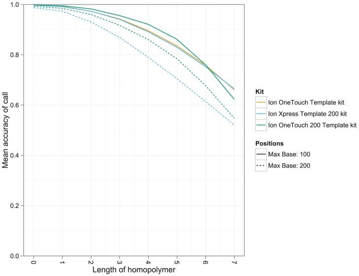
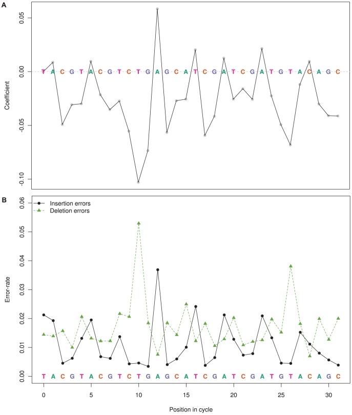
The Ion Torrent Personal Genome Machine (PGM) is a new sequencing platform that substantially differs from other sequencing technologies by measuring pH rather than light to detect polymerisation events. Using re-sequencing datasets, we comprehensively characterise the biases and errors introduced by the PGM at both the base and flow level, across a combination of factors, including chip density, sequencing kit, template species and machine. We found two distinct insertion/deletion (indel) error types that accounted for the majority of errors introduced by the PGM. The main error source was inaccurate flow-calls, which introduced indels at a raw rate of 2.84% (1.38% after quality clipping) using the OneTouch 200 bp kit. Inaccurate flow-calls typically resulted in over-called short-homopolymers and under-called long-homopolymers. Flow-call accuracy decreased with consecutive flow cycles, but we also found significant periodic fluctuations in the flow error-rate, corresponding to specific positions within the flow-cycle pattern. Another less common PGM error, high frequency indel (HFI) errors, are indels that occur at very high frequency in the reads relative to a given base position in the reference genome, but in the majority of instances were not replicated consistently across separate runs. HFI errors occur approximately once every thousand bases in the reference, and correspond to 0.06% of bases in reads. Currently, the PGM does not achieve the accuracy of competing light-based technologies. However, flow-call inaccuracy is systematic and the statistical models of flow-values developed here will enable PGM-specific bioinformatics approaches to be developed, which will account for these errors. HFI errors may prove more challenging to address, especially for polymorphism and amplicon applications, but may be overcome by sequencing the same DNA template across multiple chips.
Overview
The claims and statistics of this paper haven’t been checked yet.
Run the check — free, no account needed. It reads the open-access text and checks the sources it cites.
Integrity signals
Registry
Cites
Statistics
Figures
Verification
Claims the paper makes
The claims and statistics of this paper haven’t been checked yet.
Run the check — free, no account needed. It reads the open-access text and checks the sources it cites.
Claims other papers make about this one
Each is checked against this paper’s own text: does it say what the citing paper says it does?
The cited source says what the claim attributes to it.
In the citing paper
“The Ion Torrent system is similar to the Roche/454, and also has similar issues with indels (50).”
From Tandem repeats lead to sequence assembly errors and impose multi-level challenges for genome and protein databases (2019) · cites this paper as [50]
Self-check
Percentages, sums and reported differences re-computed from the paper’s own numbers.
The self-check needs the paper’s full text.
Citations
Cites
A Simple Sequentially Rejective Multiple Test Procedure
(1979) · Scandinavian Journal of Statistics · doi:10.2307/4615733 · Cited by 21,526
Versatile and open software for comparing large genomes
Kurtz, S., Phillippy, A., Delcher, A. L., Smoot, M., Shumway, M., Antonescu, C., & Salzberg, S. L. (2004) · Genome Biology · doi:10.1186/gb-2004-5-2-r12 · Cited by 5,254
An integrated semiconductor device enabling non-optical genome sequencing
Rothberg, J. M., Hinz, W., Rearick, T. M., Schultz, J., Mileski, W., Davey, M. S., Leamon, J. H., Johnson, K., Milgrew, M. J., Edwards, M. M., et al. (2011) · Nature · doi:10.1038/nature10242 · Cited by 2,275
Quail, M., Smith, M. E., Coupland, P., Otto, T. D., Harris, S. R., Connor, T. R., Bertoni, A., Swerdlow, H. P., & Gu, Y. (2012) · BMC Genomics · doi:10.1186/1471-2164-13-341 · Cited by 2,031 · cited 7×
“Two studies comparing benchtop sequencers, including the PGM, were recently published [2,3], both focusing on the assembly prospects of benchtop platforms on single isolate genomes.”
BackgroundMethodInfluentialRemoving Noise From Pyrosequenced Amplicons
Quince, C., Lanzen, A., Davenport, R. J., & Turnbaugh, P. J. (2011) · BMC Bioinformatics · doi:10.1186/1471-2105-12-38 · Cited by 1,592
Performance comparison of benchtop high-throughput sequencing platforms
Loman, N. J., Misra, R. V., Dallman, T. J., Constantinidou, C., Gharbia, S. E., Wain, J., & Pallen, M. J. (2012) · Nature Biotechnology · doi:10.1038/nbt.2198 · Cited by 1,337
Accuracy and quality of massively parallel DNA pyrosequencing
Huse, S. M., Huber, J. A., Morrison, H. G., Sogin, M. L., & Welch, D. M. (2007) · Genome Biology · doi:10.1186/gb-2007-8-7-r143 · Cited by 1,282
Genome evolution and adaptation in a long-term experiment with Escherichia coli
Barrick, J. E., Yu, D. S., Yoon, S. H., Jeong, H., Oh, T. K., Schneider, D., Lenski, R. E., & Kim, J. F. (2009) · Nature · doi:10.1038/nature08480 · Cited by 1,184
Analyzing and minimizing PCR amplification bias in Illumina sequencing libraries
Aird, D., Ross, M. G., Chen, W.-S., Danielsson, M., Fennell, T., Russ, C., Jaffe, D. B., Nusbaum, C., & Gnirke, A. (2011) · Genome Biology · doi:10.1186/gb-2011-12-2-r18 · Cited by 1,174
Accurate determination of microbial diversity from 454 pyrosequencing data
Quince, C., Lanzén, A., Curtis, T. P., Davenport, R. J., Hall, N., Head, I. M., Read, L. F., & Sloan, W. T. (2009) · Nature Methods · doi:10.1038/nmeth.1361 · Cited by 999
A large genome center's improvements to the Illumina sequencing system
Quail, M. A., Kozarewa, I., Smith, F., Scally, A., Stephens, P. J., Durbin, R., Swerdlow, H., & Turner, D. J. (2008) · Nature Methods · doi:10.1038/nmeth.1270 · Cited by 727
PCR fidelity of pfu DNA polymerase and other thermostable DNA polymerases
Cline, J. (1996) · Nucleic Acids Research · doi:10.1093/nar/24.18.3546 · Cited by 718
Rapidly denoising pyrosequencing amplicon reads by exploiting rank-abundance distributions
Reeder, J., & Knight, R. (2010) · Nature Methods · doi:10.1038/nmeth0910-668b · Cited by 678
Fast Mapping of Short Sequences with Mismatches, Insertions and Deletions Using Index Structures
Hoffmann, S., Otto, C., Kurtz, S., Sharma, C. M., Khaitovich, P., Vogel, J., Stadler, P. F., & Hackermüller, J. (2009) · PLoS Computational Biology · doi:10.1371/journal.pcbi.1000502 · Cited by 543
Systematic artifacts in metagenomes from complex microbial communities
Gomez‐Alvarez, V., Teal, T. K., & Schmidt, T. M. (2009) · The ISME Journal · doi:10.1038/ismej.2009.72 · Cited by 470
Accuracy and quality assessment of 454 GS-FLX Titanium pyrosequencing
Gilles, A., Meglécz, E., Pech, N., Ferreira, S., Malausa, T., & Martin, J. (2011) · BMC Genomics · doi:10.1186/1471-2164-12-245 · Cited by 377
Artificial and natural duplicates in pyrosequencing reads of metagenomic data
Niu, B., Fu, L., Sun, S., & Li, W. (2010) · BMC Bioinformatics · doi:10.1186/1471-2105-11-187 · Cited by 273
Wickham, H. (2009) · Springer eBooks · doi:10.1007/978-0-387-98141-3_1 · Cited by 258
Characteristics of 454 pyrosequencing data—enabling realistic simulation with flowsim
Balzer, S., Malde, K., Lanzén, A., Sharma, A., & Jonassen, I. (2010) · Bioinformatics · doi:10.1093/bioinformatics/btq365 · Cited by 124
Neutral Mutations and Neutral Substitutions in Bacterial Genomes
Ochman, H. (2003) · Molecular Biology and Evolution · doi:10.1093/molbev/msg229 · Cited by 95
Systematic exploration of error sources in pyrosequencing flowgram data
Balzer, S., Malde, K., & Jonassen, I. (2011) · Bioinformatics · doi:10.1093/bioinformatics/btr251 · Cited by 81
Elliott, A. M., Radecki, J., Moghis, B., et al. (2012) · Journal of Biomolecular Techniques JBT · doi:10.7171/jbt.12-2301-003 · Cited by 71
Assessment of replicate bias in 454 pyrosequencing and a multi-purpose read-filtering tool
Mariette, J., Noirot, C., & Klopp, C. (2011) · BMC Research Notes · doi:10.1186/1756-0500-4-149 · Cited by 53
Cited by
A universal SNP and small-indel variant caller using deep neural networks
Poplin, R., Chang, P.-C., Alexander, D., Schwartz, S., Colthurst, T., Ku, A., Newburger, D., Dijamco, J., Nguyen, N., Afshar, P. T., et al. (2018) · Nature Biotechnology · doi:10.1038/nbt.4235 · Cited by 1,840
Tørresen, O. K., Star, B., Mier, P., Andrade-Navarro, M. A., Bateman, A., Jarnot, P., Gruca, A., Grynberg, M., Kajava, A. V., Promponas, V. J., et al. (2019) · Nucleic Acids Research · doi:10.1093/nar/gkz841 · Cited by 347
Historical perspective, development and applications of next-generation sequencing in plant virology
Barba, M., Czosnek, H., & Hadidi, A. (2014) · Viruses · doi:10.3390/v6010106 · Cited by 317
“38 [26]”
Couraud, S., Vaca-Paniagua, F., Villar, S., Oliver, J., Schuster, T., Blanché, H., Girard, N., Trédaniel, J., Guilleminault, L., Gervais, R., et al. (2014) · Clinical Cancer Research · doi:10.1158/1078-0432.ccr-13-3063 · Cited by 215
Detecting and correcting systematic variation in large-scale RNA sequencing data
Li, S., Łabaj, P. P., Zumbo, P., Sykacek, P., Shi, W., Shi, L., Phan, J., Wu, P.-Y., Wang, M., Wang, C., et al. (2014) · Nature Biotechnology · doi:10.1038/nbt.3000 · Cited by 175
Metadata
- Authors
- Bragg, L. M., Stone, G., Butler, M. K., Hugenholtz, P., & Tyson, G. W.
- Venue
- PLoS Computational Biology
- Publisher
- Public Library of Science (PLoS)
- Published
- 2013-04-11
- Volume
- 9
- Issue
- 4
- Pages
- e1003031
- ISSN
- 1553-7358
- PMC
- PMC3623719
- Cited by
- 261
- References
- 23
- Language
- en
About these checks
Registry, retraction, Cites and statistics results are computed, not judged, with one exception: a printed reference that no index lists is read once by a model before it counts as a citation error. Claims are extracted by a model and kept only when their quote appears verbatim in the text; each cited source is then checked, with a model’s help, for whether it says what the claim relies on. Those verdicts can be wrong — read the claim’s quote and the cited source before relying on one.
Statistics and arithmetic are recomputed, not judged.
Confidence bands are shown only for fields calibrated on our annotated test set. None is calibrated yet, so no band is shown.
What counts as a claim ›How we measure confidence ›How we check this ›
Are you an author, or do you see a problem with this page? Request a review
Data sources
Bibliographic data: Semantic Scholar, OpenAlex, Crossref.
Contains information from the Semantic Scholar Academic Graph Datasets, made available under the ODC Attribution License (ODC-BY 1.0).
Semantic Scholar’s data is described in: Kinney, R., et al. (2023). The Semantic Scholar Open Data Platform. arXiv:2301.10140.
