

The DOI matches its Crossref record; 61 of the 61 references it cites were found in a registry or an index.
Eliciting priors and relaxing the single causal variant assumption in colocalisation analyses
Open accessPublished version of a preprint
Abstract
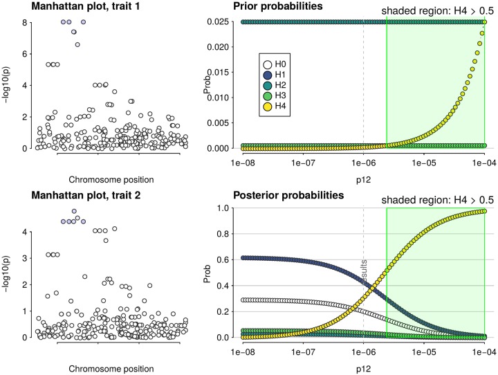
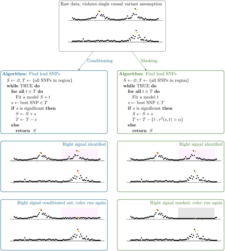
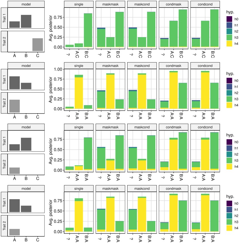
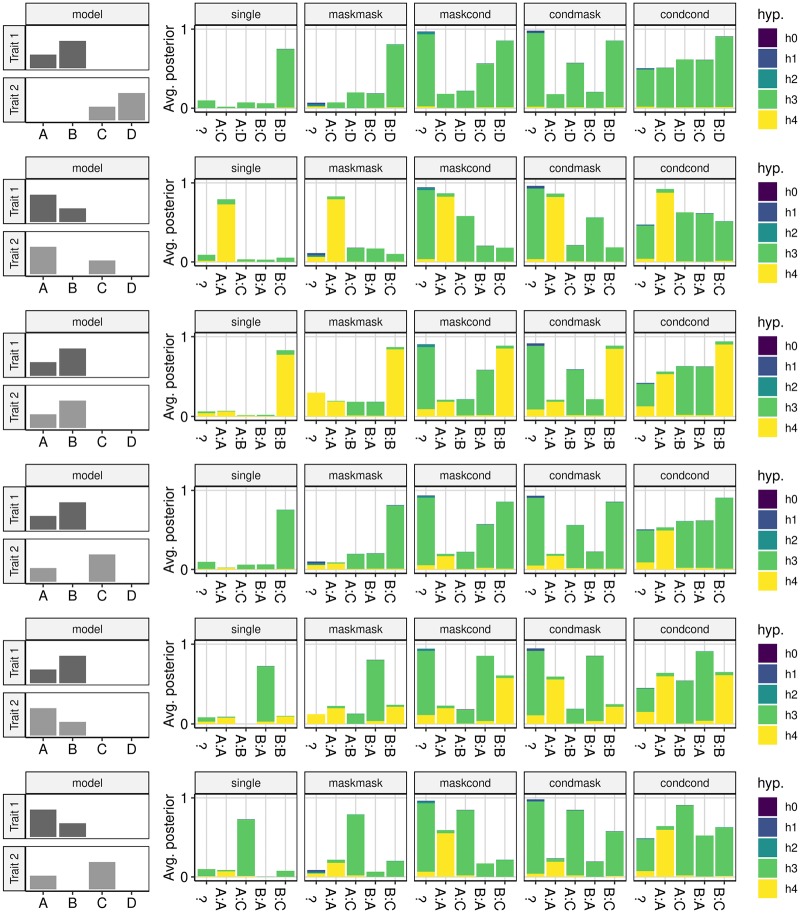
Horizontal integration of summary statistics from different GWAS traits can be used to evaluate evidence for their shared genetic causality. One popular method to do this is a Bayesian method, coloc, which is attractive in requiring only GWAS summary statistics and no linkage disequilibrium estimates and is now being used routinely to perform thousands of comparisons between traits. Here we show that while most users do not adjust default software values, misspecification of prior parameters can substantially alter posterior inference. We suggest data driven methods to derive sensible prior values, and demonstrate how sensitivity analysis can be used to assess robustness of posterior inference. The flexibility of coloc comes at the expense of an unrealistic assumption of a single causal variant per trait. This assumption can be relaxed by stepwise conditioning, but this requires external software and an LD matrix aligned to study alleles. We have now implemented conditioning within coloc, and propose a new alternative method, masking, that does not require LD and approximates conditioning when causal variants are independent. Importantly, masking can be used in combination with conditioning where allelically aligned LD estimates are available for only a single trait. We have implemented these developments in a new version of coloc which we hope will enable more informed choice of priors and overcome the restriction of the single causal variant assumptions in coloc analysis.
Overview
The claims and statistics of this paper haven’t been checked yet.
Run the check — free, no account needed. It reads the open-access text and checks the sources it cites.
Integrity signals
Registry
Cites
Statistics
Figures
Verification
Claims the paper makes
The claims and statistics of this paper haven’t been checked yet.
Run the check — free, no account needed. It reads the open-access text and checks the sources it cites.
Claims other papers make about this one
Each is checked against this paper’s own text: does it say what the citing paper says it does?
In the citing paper
“Alternatively, Bayesian frameworks for colocalization analysis consider GWAS summary statistics for both traits across multiple SNPs in the region around the IV and assess either the evidence that each variant is jointly causal115 or consider shared causal variants as one of five competing hypotheses.116”
From Mendelian randomization (2022) · cites this paper as [116]
Self-check
Percentages, sums and reported differences re-computed from the paper’s own numbers.
The self-check needs the paper’s full text.
Citations
Cites
The MR-Base platform supports systematic causal inference across the human phenome
Hemani, G., Zheng, J., Elsworth, B., Wade, K. H., Haberland, V., Baird, D., Laurin, C., Burgess, S., Bowden, J., Langdon, R., et al. (2018) · eLife · doi:10.7554/elife.34408 · Cited by 7,959
Davey Smith, G., & Ebrahim, S. (2003) · International Journal of Epidemiology · doi:10.1093/ije/dyg070 · Cited by 5,882
LD Score regression distinguishes confounding from polygenicity in genome-wide association studies
Schizophrenia Working Group of the Psychiatric Genomics Consortium, Bulik-Sullivan, B. K., Loh, P.-R., Finucane, H. K., Ripke, S., Yang, J., Patterson, N., Daly, M. J., Price, A. L., & Neale, B. M. (2015) · Nature Genetics · doi:10.1038/ng.3211 · Cited by 5,559
Giambartolomei, C., Vukcevic, D., Schadt, E. E., Franke, L., Hingorani, A. D., Wallace, C., & Plagnol, V. (2014) · PLoS Genetics · doi:10.1371/journal.pgen.1004383 · Cited by 4,261
Self-citationGenetic effects on gene expression across human tissues
GTEx Consortium (2017) · Nature · doi:10.1038/nature24277 · Cited by 4,036
Buniello, A., MacArthur, J. A. L., Cerezo, M., Harris, L. W., Hayhurst, J., Malangone, C., McMahon, A., Morales, J., Mountjoy, E., Sollis, E., et al. (2019) · Nucleic Acids Research · doi:10.1093/nar/gky1120 · Cited by 4,000
10 Years of GWAS Discovery: Biology, Function, and Translation
Visscher, P. M., Wray, N. R., Zhang, Q., Sklar, P., McCarthy, M. I., Brown, M. A., & Yang, J. (2017) · The American Journal of Human Genetics · doi:10.1016/j.ajhg.2017.06.005 · Cited by 3,719
Integration of summary data from GWAS and eQTL studies predicts complex trait gene targets
Zhu, Z., Zhang, F., Hu, H., Bakshi, A., Robinson, M. R., Powell, J. E., Montgomery, G. W., Goddard, M. E., Wray, N. R., Visscher, P. M., et al. (2016) · Nature Genetics · doi:10.1038/ng.3538 · Cited by 3,352
An Expanded View of Complex Traits: From Polygenic to Omnigenic
Boyle, E. A., Li, Y. I., & Pritchard, J. K. (2017) · Cell · doi:10.1016/j.cell.2017.05.038 · Cited by 2,851
Integrative approaches for large-scale transcriptome-wide association studies
Gusev, A., Ko, A., Shi, H., Bhatia, G., Chung, W., Penninx, B. W. J. H., Jansen, R., de Geus, E. J. C., Boomsma, D. I., Wright, F. A., et al. (2016) · Nature Genetics · doi:10.1038/ng.3506 · Cited by 2,479
Cited by
Sorted by citations
Sanderson, E., Glymour, M. M., Holmes, M. V., Kang, H., Morrison, J., Munafò, M. R., Palmer, T., Schooling, C. M., Wallace, C., Zhao, Q., et al. (2022) · Nature Reviews Methods Primers · doi:10.1038/s43586-021-00092-5 · Cited by 2,229
Self-citationWightman, D. P., Jansen, I. E., Savage, J. E., Shadrin, A. A., Bahrami, S., Holland, D., Rongve, A., Børte, S., Winsvold, B. S., Drange, O. K., et al. (2021) · Nature Genetics · doi:10.1038/s41588-021-00921-z · Cited by 1,011
A more accurate method for colocalisation analysis allowing for multiple causal variants
Wallace, C. (2021) · PLOS Genetics · doi:10.1371/journal.pgen.1009440 · Cited by 567
Self-citationFoley, C. N., Staley, J. R., Breen, P. G., Sun, B. B., Kirk, P., Burgess, S., & Howson, J. M. M. (2021) · Nature Communications · doi:10.1038/s41467-020-20885-8 · Cited by 552
Zuber, V., Grinberg, N. F., Gill, D., Manipur, I., Slob, E. A. W., Patel, A., Wallace, C., & Burgess, S. (2022) · The American Journal of Human Genetics · doi:10.1016/j.ajhg.2022.04.001 · Cited by 532
Self-citation
Metadata
- Authors
- Wallace, C.
- Affiliations
- University of Cambridge (GB)
- Corresponding author
- Wallace, Chris
- ORCID
- Wallace, Chris
- Venue
- PLOS Genetics
- Publisher
- Public Library of Science (PLoS)
- Published
- 2020-04-20
- Volume
- 16
- Issue
- 4
- Pages
- e1008720
- ISSN
- 1553-7390 (ISSN-L)
- 1553-7404
- PMC
- PMC7192519
- OpenAlex
- W3016489931
- Cited by
- 441
- References
- 59
- Citations by year
- 2026: 75 · 2025: 98 · 2024: 123 · 2023: 47 · 2022: 39 · 2021: 43 · 2020: 15
- FWCI
- 21.26
- Type
- journal article
- Language
- en
- Update notices
- Open access
- gold
- doi.org
- Licence
- Locations
- PLoS Genetics (publishedVersion, cc-by)
- bioRxiv (Cold Spring Harbor Laboratory) (acceptedVersion, cc-by)
- PubMed Central (publishedVersion, cc-by)
- PubMed (publishedVersion)
- RePEc: Research Papers in Economics (submittedVersion)
- DOAJ (DOAJ: Directory of Open Access Journals) (submittedVersion, cc-by-sa)
- Figshare (submittedVersion, cc-by)
- Apollo (University of Cambridge) (submittedVersion, cc-by)
- Apollo (cc-by)
- Funders
- Wellcome Trust (WT107881)
- Medical Research Council (MC UU 00002/4)
- Topics
- Life Sciences › Biochemistry, Genetics and Molecular Biology › Genetics › Genetic Associations and Epidemiology
- Life Sciences › Biochemistry, Genetics and Molecular Biology › Genetics › Genetic Mapping and Diversity in Plants and Animals
- Life Sciences › Biochemistry, Genetics and Molecular Biology › Genetics › Genetic and phenotypic traits in livestock
- Keywords
- COLOC, prior specification, prior distributions, sensitivity analysis, masking, linkage disequilibrium, GWAS summary statistics
- MeSH terms
- Humans, Linkage Disequilibrium, Polymorphism, Single Nucleotide, Quantitative Trait Loci, Genome-Wide Association Study
About these checks
Registry, retraction, Cites and statistics results are computed, not judged, with one exception: a printed reference that no index lists is read once by a model before it counts as a citation error. Claims are extracted by a model and kept only when their quote appears verbatim in the text; each cited source is then checked, with a model’s help, for whether it says what the claim relies on. Those verdicts can be wrong — read the claim’s quote and the cited source before relying on one.
Statistics and arithmetic are recomputed, not judged.
Confidence bands are shown only for fields calibrated on our annotated test set. None is calibrated yet, so no band is shown.
What counts as a claim ›How we measure confidence ›How we check this ›
Are you an author, or do you see a problem with this page? Request a review
