Cited by 810Blind Source Separation TechniquesEEG and Brain-Computer InterfacesTensor decomposition and applications

The DOI matches its Crossref record; 56 of the 57 references it cites were found in a registry or an index.

Independent EEG Sources Are Dipolar

Open access
Delorme, Arnaud, Palmer, Jason, Onton, Julie, Oostenveld, Robert, Makeig, Scott·2012·PLoS ONE

Abstract

Independent component analysis (ICA) and blind source separation (BSS) methods are increasingly used to separate individual brain and non-brain source signals mixed by volume conduction in electroencephalographic (EEG) and other electrophysiological recordings. We compared results of decomposing thirteen 71-channel human scalp EEG datasets by 22 ICA and BSS algorithms, assessing the pairwise mutual information (PMI) in scalp channel pairs, the remaining PMI in component pairs, the overall mutual information reduction (MIR) effected by each decomposition, and decomposition 'dipolarity' defined as the number of component scalp maps matching the projection of a single equivalent dipole with less than a given residual variance. The least well-performing algorithm was principal component analysis (PCA); best performing were AMICA and other likelihood/mutual information based ICA methods. Though these and other commonly-used decomposition methods returned many similar components, across 18 ICA/BSS algorithms mean dipolarity varied linearly with both MIR and with PMI remaining between the resulting component time courses, a result compatible with an interpretation of many maximally independent EEG components as being volume-conducted projections of partially-synchronous local cortical field activity within single compact cortical domains. To encourage further method comparisons, the data and software used to prepare the results have been made available (http://sccn.ucsd.edu/wiki/BSSComparison).

Overview

The claims and statistics of this paper haven’t been checked yet.

Run the check — free, no account needed. It reads the open-access text and checks the sources it cites.

A few free checks a day · papers already verified open instantly · results are public

Integrity signals

Registry

Crossref · 10.1371/journal.pone.0030135

Cites

56 of 56 references verified0 citation errors · 0 not checkable

Statistics

Figures

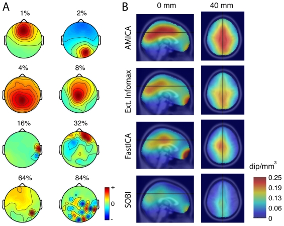
Figure 1 Component dipolarity and equivalent dipole density. A. Example component scalp maps more (top) to less (bottom) resembling the projection of a single equivalent dipole. Eight interpolated independent component (IC) scalp maps with progressively more difference from the projection of the best-fitting equivalent dipole (ED) (percent of residual variance (r.v.) indicated for each map). All but the bottom-right component scalp map are from AMICA decompositions. 1st row: (left) frontal midline IC with prominent theta band activity; (right) right parietal IC with a more tangentially oriented ED model and prominent alpha band peak. 2nd row: (left) central parietal IC likely reflecting coupled field activity in adjacent left and right medial cortex; (right) more anterior midline IC. 3rd row: (left) IC accounting for EMG activity of a right post-auricular muscle; (right) IC of uncertain origin. 4th row: (left) IC accounting for electrode noise at the most affected (red) scalp electrode; (right) high-order PCA component with a characteristic ‘checkerboard’ scalp map unlike the projection of any single ED. B. Mean (left) medial sagittal and (right) axial (z = 40 mm) densities of near-dipolar (r.v.< = 5%) component equivalent dipoles across all data sets, from four (indicated) decomposition methods.
Figure 1 Component dipolarity and equivalent dipole density. A. Example component scalp maps more (top) to less (bottom) resembling the projection of a single equivalent dipole. Eight interpolated independent component (IC) scalp maps with progressively more difference from the projection of the best-fitting equivalent dipole (ED) (percent of residual variance (r.v.) indicated for each map). All but the bottom-right component scalp map are from AMICA decompositions. 1st row: (left) frontal midline IC with prominent theta band activity; (right) right parietal IC with a more tangentially oriented ED model and prominent alpha band peak. 2nd row: (left) central parietal IC likely reflecting coupled field activity in adjacent left and right medial cortex; (right) more anterior midline IC. 3rd row: (left) IC accounting for EMG activity of a right post-auricular muscle; (right) IC of uncertain origin. 4th row: (left) IC accounting for electrode noise at the most affected (red) scalp electrode; (right) high-order PCA component with a characteristic ‘checkerboard’ scalp map unlike the projection of any single ED. B. Mean (left) medial sagittal and (right) axial (z = 40 mm) densities of near-dipolar (r.v.< = 5%) component equivalent dipoles across all data sets, from four (indicated) decomposition methods.CC BY · PubMed Central
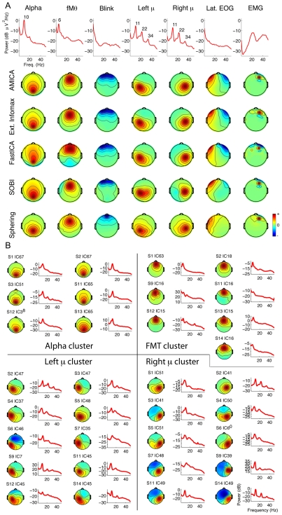
Figure 2 ICA algorithms return similar dipolar components. A. The top rows show activity spectra and scalp maps for seven AMICA components from one subject accounting respectively for eye blinks, lateral eye movements (EOG), and right frontal scalp muscle activity as well as posterior alpha band, central mu rhythm, and frontal midline theta activity. Lower four rows show scalp maps of best-matching components by Extended Infomax ICA, FastICA, SOBI, and sphering decompositions of the same subject data, e.g., those with highest absolute scalp map correlations to the respective AMICA components. Note the resemblance of the scalp maps in each case for AMICA and Extended Infomax, and the differences between the AMICA and sphering component maps. B. Scalp maps and mean activity spectra of four clusters of similar AMICA components from 6–10 different data sets from different subjects, isolated by visual inspection of component scalp maps and mean activity spectra and accounting respectively for central occipital alpha, frontal midline theta, and left and right mu rhythm activities.
Figure 2 ICA algorithms return similar dipolar components. A. The top rows show activity spectra and scalp maps for seven AMICA components from one subject accounting respectively for eye blinks, lateral eye movements (EOG), and right frontal scalp muscle activity as well as posterior alpha band, central mu rhythm, and frontal midline theta activity. Lower four rows show scalp maps of best-matching components by Extended Infomax ICA, FastICA, SOBI, and sphering decompositions of the same subject data, e.g., those with highest absolute scalp map correlations to the respective AMICA components. Note the resemblance of the scalp maps in each case for AMICA and Extended Infomax, and the differences between the AMICA and sphering component maps. B. Scalp maps and mean activity spectra of four clusters of similar AMICA components from 6–10 different data sets from different subjects, isolated by visual inspection of component scalp maps and mean activity spectra and accounting respectively for central occipital alpha, frontal midline theta, and left and right mu rhythm activities.CC BY · PubMed Central
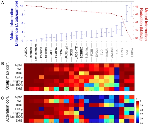
Figure 3 Correlations of component scalp maps and time courses across algorithms for the seven identified component types. A. (Blue trace) Mean (±std. deviation across all data sets) additional mutual information remaining in the time courses of components returned by each of the 22 decomposition algorithms relative to AMICA decompositions of the same data, sorted left to right by overall degree of mutual information reduction (MIR, red trace). Names of the 12 algorithms returning components with more mutual information reduction (MIR) than simple sphering (bottom left) are lettered in black. B. Mean correlations between seven representative AMICA component scalp maps from one participant (same as top row in Figure 2 ) and the seven components with best absolute scalp map correlations to these returned by the other decompositions of this subject's data. C. Mean correlations between the independent component activation time courses for the same component pairs as in B. Although the time course correlations are generally lower than scalp map correlations, the two patterns of results are similar, with (leftmost) decompositions effecting the most mutual information reduction returning components whose scalp maps and activities generally strongly resemble the selected AMICA components.
Figure 3 Correlations of component scalp maps and time courses across algorithms for the seven identified component types. A. (Blue trace) Mean (±std. deviation across all data sets) additional mutual information remaining in the time courses of components returned by each of the 22 decomposition algorithms relative to AMICA decompositions of the same data, sorted left to right by overall degree of mutual information reduction (MIR, red trace). Names of the 12 algorithms returning components with more mutual information reduction (MIR) than simple sphering (bottom left) are lettered in black. B. Mean correlations between seven representative AMICA component scalp maps from one participant (same as top row in Figure 2 ) and the seven components with best absolute scalp map correlations to these returned by the other decompositions of this subject's data. C. Mean correlations between the independent component activation time courses for the same component pairs as in B. Although the time course correlations are generally lower than scalp map correlations, the two patterns of results are similar, with (leftmost) decompositions effecting the most mutual information reduction returning components whose scalp maps and activities generally strongly resemble the selected AMICA components.CC BY · PubMed Central
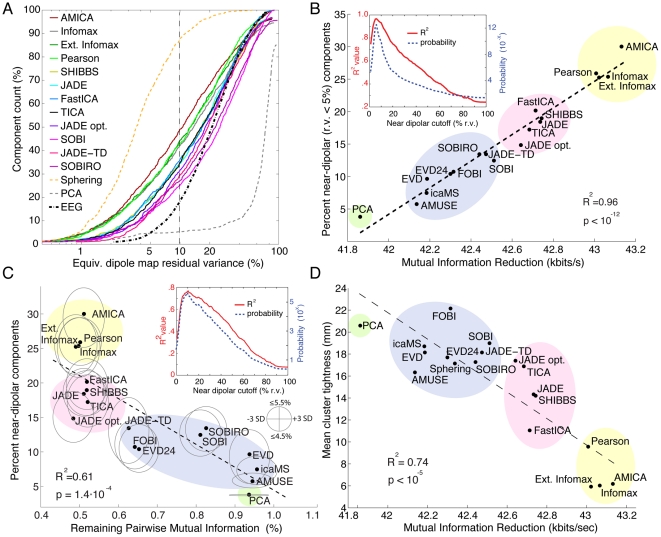
Figure 4 Decompositions that reduce total mutual information in the component time courses also return more components with near-dipolar scalp maps. A. Cumulative mean percentage of components returned by each blind source separation algorithm sorted by percent scalp map residual variance (r.v.) remaining after subtracting the best-fitting single equivalent dipole model. The key lists the decomposition methods in order of their mean number of near-dipolar components (e.g, having scalp map r.v.< = 10%). Note the topmost yellow dashed trace (sphering), the bottommost trace (PCA, principal component analysis), and the black dashed trace (mean cumulative dipolarity of 71 sample EEG scalp maps randomly selected from each dataset). B. (Ordinate) percentage of components with strongly dipolar scalp maps (r.v.< = 5%), plotted against (abscissa) mean mutual information reduction (MIR) for 18 of the algorithms. The dashed line shows the linear regression (R2 = 0.96, p<10−12). Figure inset: (red trace) Probability that MIR varies linearly with the proportion of near-dipolar components, and (blue) proportion of variance accounted for by the linear fit, as functions of ‘near-dipolar’ r.v. threshold. Both variables peak at a ‘dipolar’ residual variance cutoff of 6%. The 18 decomposition methods form four groups (colored oval highlights added manually to group algorithms by type; see Methods). The computed standard deviations of these MI values are too small to be represented. C. Percentage near-dipolar components (with scalp map r.v.< = 5%) as a function of mean percentage of channel pairwise mutual information (PMI) remaining between component time courses. Ellipses around each data point indicate, on the horizontal axis, 3-std. dev. confidence bounds for each component PMI calculation. Note: the PMI standard error of the mean (SEM) confidence region is ∼180 times more narrow. The heights of the ovals show the range of decomposition ‘dipolarity’ values for neighborhood r.v. cutoff values between 4.5% and 5.5% ; other details as in B. D. For the seven identified component clusters for each decomposition method (as in Figure 2 ), component cluster tightness (CCT) was defined as mean distance from each component equivalent dipole to the method cluster dipole centroid. As expected, mean CCT was smallest for AMICA. Across all decomposition methods, the relationship between cluster tightness and MIR again had a near linear trend (r2 = 0.74). Thus, in general decompositions producing more MIR also returned components of seven identified types with more consistent equivalent dipole locations across subjects.
Figure 4 Decompositions that reduce total mutual information in the component time courses also return more components with near-dipolar scalp maps. A. Cumulative mean percentage of components returned by each blind source separation algorithm sorted by percent scalp map residual variance (r.v.) remaining after subtracting the best-fitting single equivalent dipole model. The key lists the decomposition methods in order of their mean number of near-dipolar components (e.g, having scalp map r.v.< = 10%). Note the topmost yellow dashed trace (sphering), the bottommost trace (PCA, principal component analysis), and the black dashed trace (mean cumulative dipolarity of 71 sample EEG scalp maps randomly selected from each dataset). B. (Ordinate) percentage of components with strongly dipolar scalp maps (r.v.< = 5%), plotted against (abscissa) mean mutual information reduction (MIR) for 18 of the algorithms. The dashed line shows the linear regression (R2 = 0.96, p<10−12). Figure inset: (red trace) Probability that MIR varies linearly with the proportion of near-dipolar components, and (blue) proportion of variance accounted for by the linear fit, as functions of ‘near-dipolar’ r.v. threshold. Both variables peak at a ‘dipolar’ residual variance cutoff of 6%. The 18 decomposition methods form four groups (colored oval highlights added manually to group algorithms by type; see Methods). The computed standard deviations of these MI values are too small to be represented. C. Percentage near-dipolar components (with scalp map r.v.< = 5%) as a function of mean percentage of channel pairwise mutual information (PMI) remaining between component time courses. Ellipses around each data point indicate, on the horizontal axis, 3-std. dev. confidence bounds for each component PMI calculation. Note: the PMI standard error of the mean (SEM) confidence region is ∼180 times more narrow. The heights of the ovals show the range of decomposition ‘dipolarity’ values for neighborhood r.v. cutoff values between 4.5% and 5.5% ; other details as in B. D. For the seven identified component clusters for each decomposition method (as in Figure 2 ), component cluster tightness (CCT) was defined as mean distance from each component equivalent dipole to the method cluster dipole centroid. As expected, mean CCT was smallest for AMICA. Across all decomposition methods, the relationship between cluster tightness and MIR again had a near linear trend (r2 = 0.74). Thus, in general decompositions producing more MIR also returned components of seven identified types with more consistent equivalent dipole locations across subjects.CC BY · PubMed Central
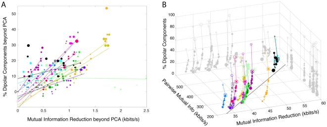
Figure 5 Channel pair-wise mutual information, mutual information reduction, and dipolarity for each dataset and algorithm. A. For each data set and decomposition, mutual information reduction versus difference in the percentage of near-dipolar components (less than 5% residual variance) and the (nearly always lower) percentage produced by PCA. The size of the disk markers is proportional to the number of components whose scalp maps are near the 5% r.v. threshold (in the range 4.5% to 5.5%). Colors group results for each dataset. For each dataset, a linear fit based on all 18 decompositions (excluding sphering) is shown by a straight line. Best-fitting lines for all datasets but one (light green) have a positive slope as in Figure 4B (p<10−5 by two-tailed parametric unpaired t-test; df = 12). B. The percentage of dipolar components (vertical axis) in each decomposition, versus (left-going axis) the initial mutual information in the channel data for each data set as estimated by total channel pairwise mutual information (PMI), and (right-going axis) the overall reduction in mutual information (MIR) effected by the decomposition. The linear trend across datasets (indicated by the best-fitting line drawn on the ‘floor’ of the plotting box) shows that as might be expected, the more (pairwise) mutual information in the channel data, the more mutual information was removed by all decompositions. Results for the 18 algorithms in Figure 4 , plus sphering, are connected in order of mean mutual information reduction (MIR) in Figure 4A . Results of AMICA decomposition (crossed circles) are connected by a dashed line to those for sphering (empty circles). Sphering produced more near-dipolar components that the other ICA/BSS algorithms, but produced less mutual information reduction than ICA algorithms, while as expected returning components having scalp maps centered on each electrode location (compare Fig. 2A).
Figure 5 Channel pair-wise mutual information, mutual information reduction, and dipolarity for each dataset and algorithm. A. For each data set and decomposition, mutual information reduction versus difference in the percentage of near-dipolar components (less than 5% residual variance) and the (nearly always lower) percentage produced by PCA. The size of the disk markers is proportional to the number of components whose scalp maps are near the 5% r.v. threshold (in the range 4.5% to 5.5%). Colors group results for each dataset. For each dataset, a linear fit based on all 18 decompositions (excluding sphering) is shown by a straight line. Best-fitting lines for all datasets but one (light green) have a positive slope as in Figure 4B (p<10−5 by two-tailed parametric unpaired t-test; df = 12). B. The percentage of dipolar components (vertical axis) in each decomposition, versus (left-going axis) the initial mutual information in the channel data for each data set as estimated by total channel pairwise mutual information (PMI), and (right-going axis) the overall reduction in mutual information (MIR) effected by the decomposition. The linear trend across datasets (indicated by the best-fitting line drawn on the ‘floor’ of the plotting box) shows that as might be expected, the more (pairwise) mutual information in the channel data, the more mutual information was removed by all decompositions. Results for the 18 algorithms in Figure 4 , plus sphering, are connected in order of mean mutual information reduction (MIR) in Figure 4A . Results of AMICA decomposition (crossed circles) are connected by a dashed line to those for sphering (empty circles). Sphering produced more near-dipolar components that the other ICA/BSS algorithms, but produced less mutual information reduction than ICA algorithms, while as expected returning components having scalp maps centered on each electrode location (compare Fig. 2A).CC BY · PubMed Central

Verification

Claims the paper makes

The claims and statistics of this paper haven’t been checked yet.

Run the check — free, no account needed. It reads the open-access text and checks the sources it cites.

A few free checks a day · papers already verified open instantly · results are public

Claims other papers make about this one

Each is checked against this paper’s own text: does it say what the citing paper says it does?

Self-check

Percentages, sums and reported differences re-computed from the paper’s own numbers.

The self-check needs the paper’s full text.

Citations

Cites

Show all 57 references

Research works printed but not linked: 2

  1. G Gómez-Herrero, 2008, Gómez-Herrero G, Atienza M, Egiazarian K, Cantero JL., Neuroimage, 43, 497
  2. Z Akalin Acar, 2011, Adaptive mixture independent component analysis and source localization in epilepsy., IEEE EMBC

Cited by

Sorted by citations

See all 810

Metadata

Authors
Delorme, A., Palmer, J., Onton, J., Oostenveld, R., & Makeig, S.
Affiliations
  • University of California San Diego (US)
  • Radboud University Nijmegen (NL)
Venue
PLoS ONE
Published
2012-02-15
Volume
7
Issue
2
Pages
e30135
ISSN
1932-6203 (ISSN-L)
OpenAlex
W2171746332
Cited by
810
References
57
Citations by year
2026: 34 · 2025: 47 · 2024: 50 · 2023: 58 · 2022: 80 · 2021: 76 · 2020: 80 · 2019: 67 · 2018: 68 · 2017: 56 · 2016: 50 · 2015: 48 · 2014: 48 · 2013: 32 · 2012: 15
FWCI
58.25
Type
journal article
Language
en
Open access
Locations
  • PLoS ONE (publishedVersion, cc-by)
  • Europe PMC (PubMed Central) (publishedVersion, cc-by)
  • PubMed Central (publishedVersion, cc-by)
  • PubMed (publishedVersion)
  • eScholarship (California Digital Library) (submittedVersion, cc-by)
  • HAL (submittedVersion, other-oa)
  • RePEc: Research Papers in Economics (submittedVersion)
  • DOAJ (DOAJ: Directory of Open Access Journals) (submittedVersion, cc-by-sa)
  • eScholarship (California Digital Library) (submittedVersion)
Funders
  • National Science Foundation (0613595)
  • National Institute of Mental Health (NS047293)
  • National Institute of Neurological Disorders and Stroke (R01-NS047293-01A1, R01NS047293)
Topics
  • Physical Sciences › Computer Science › Signal Processing › Blind Source Separation Techniques
  • Life Sciences › Neuroscience › Cognitive Neuroscience › EEG and Brain-Computer Interfaces
  • Physical Sciences › Mathematics › Computational Mathematics › Tensor decomposition and applications
Keywords
independent component analysis, blind source separation, EEG source localization, dipole modeling, volume conduction, mutual information, principal component analysis, scalp EEG
MeSH terms
Algorithms, Brain, Brain Mapping, Computer Simulation, Electroencephalography, Humans, Scalp, Signal Processing, Computer-Assisted, Principal Component Analysis

About these checks

Registry, retraction, Cites and statistics results are computed, not judged, with one exception: a printed reference that no index lists is read once by a model before it counts as a citation error. Claims are extracted by a model and kept only when their quote appears verbatim in the text; each cited source is then checked, with a model’s help, for whether it says what the claim relies on. Those verdicts can be wrong — read the claim’s quote and the cited source before relying on one.

Statistics and arithmetic are recomputed, not judged.

Confidence bands are shown only for fields calibrated on our annotated test set. None is calibrated yet, so no band is shown.

What counts as a claim ›How we measure confidence ›How we check this ›

Are you an author, or do you see a problem with this page? Request a review