

The DOI matches its Crossref record; 43 of the 43 references it cites were found in a registry or an index.
Effects of GC Bias in Next-Generation-Sequencing Data on De Novo Genome Assembly
Open accessAbstract
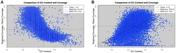
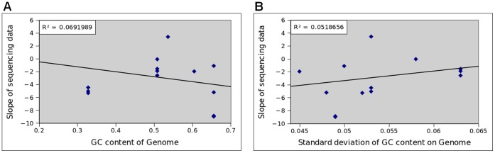
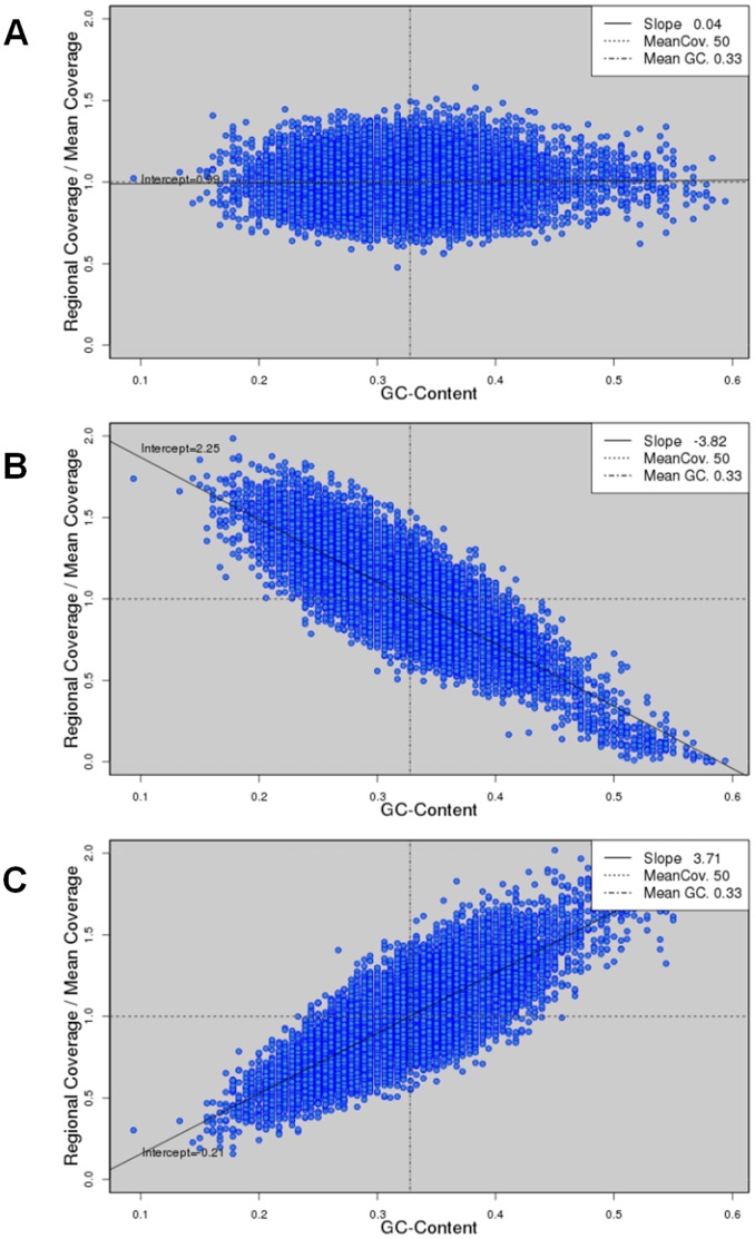
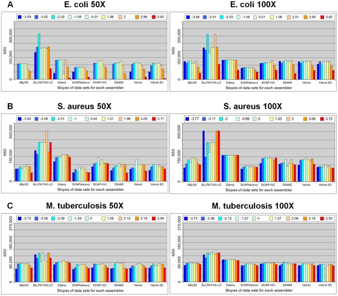
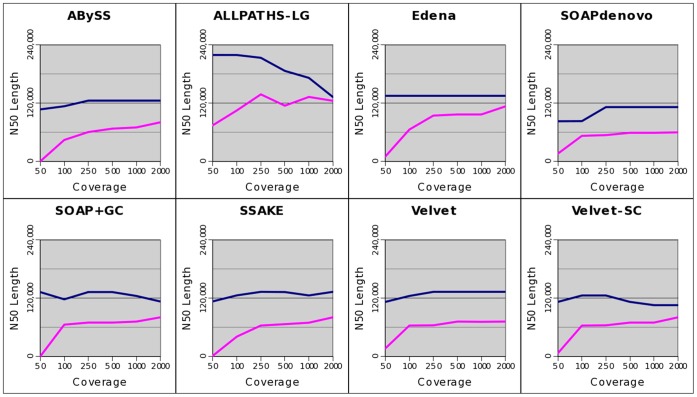
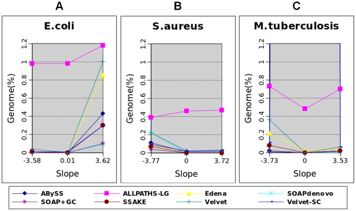
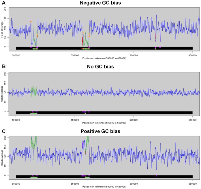
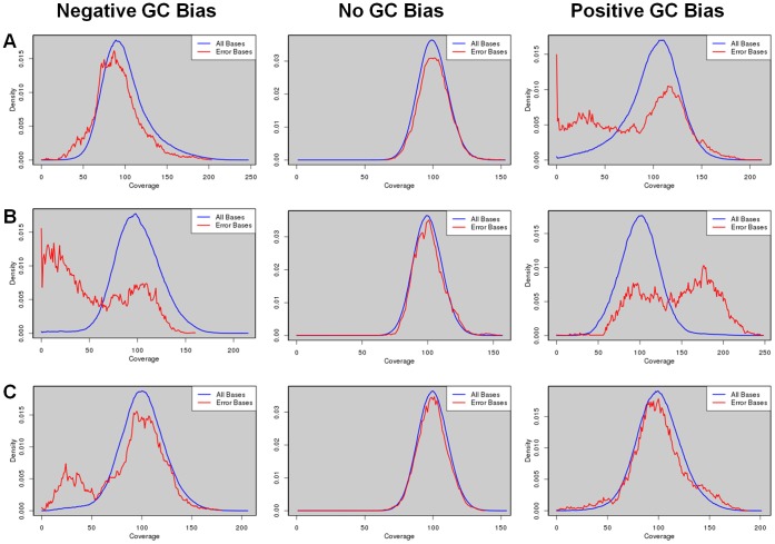
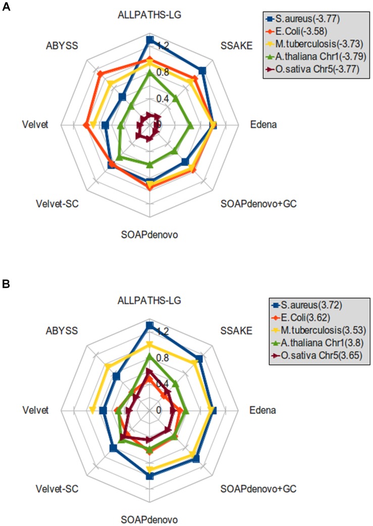
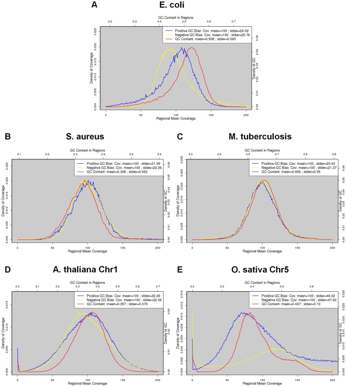
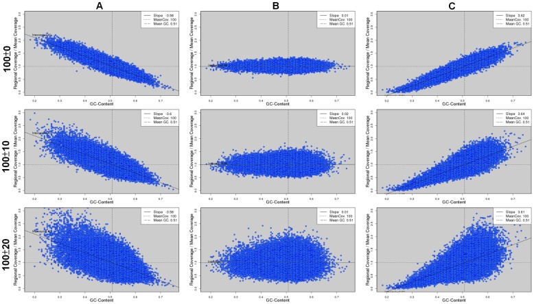
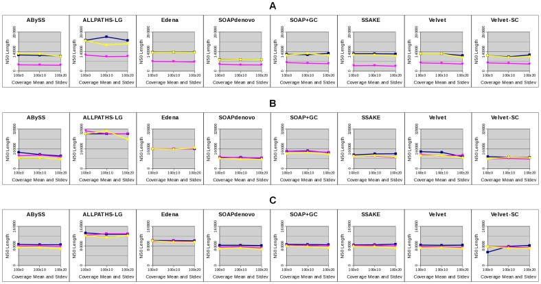
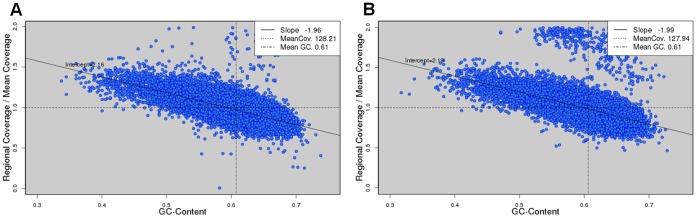
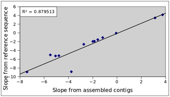
Next-generation-sequencing (NGS) has revolutionized the field of genome assembly because of its much higher data throughput and much lower cost compared with traditional Sanger sequencing. However, NGS poses new computational challenges to de novo genome assembly. Among the challenges, GC bias in NGS data is known to aggravate genome assembly. However, it is not clear to what extent GC bias affects genome assembly in general. In this work, we conduct a systematic analysis on the effects of GC bias on genome assembly. Our analyses reveal that GC bias only lowers assembly completeness when the degree of GC bias is above a threshold. At a strong GC bias, the assembly fragmentation due to GC bias can be explained by the low coverage of reads in the GC-poor or GC-rich regions of a genome. This effect is observed for all the assemblers under study. Increasing the total amount of NGS data thus rescues the assembly fragmentation because of GC bias. However, the amount of data needed for a full rescue depends on the distribution of GC contents. Both low and high coverage depths due to GC bias lower the accuracy of assembly. These pieces of information provide guidance toward a better de novo genome assembly in the presence of GC bias.
Overview
The claims and statistics of this paper haven’t been checked yet.
Run the check — free, no account needed. It reads the open-access text and checks the sources it cites.
Integrity signals
Registry
Cites
Statistics
Figures
Verification
Claims the paper makes
The claims and statistics of this paper haven’t been checked yet.
Run the check — free, no account needed. It reads the open-access text and checks the sources it cites.
Claims other papers make about this one
Each is checked against this paper’s own text: does it say what the citing paper says it does?
The cited source says what the claim attributes to it.
In the citing paper
“Illumina sequencing was previously observed to have bias on GC-extreme sequences15,27,28, but GC content in our files did not show practically significant bias in the PCR GC bias test. Therefore, high-throughput sequencing and sample dilution are modeled using random sampling.”
From Quantifying Molecular Bias in DNA Data Storage (2019) · cites this paper as [27]
Self-check
Percentages, sums and reported differences re-computed from the paper’s own numbers.
The self-check needs the paper’s full text.
Citations
Cites
Database resources of the National Center for Biotechnology Information: update
Wheeler, D. L. (2003) · Nucleic Acids Research · doi:10.1093/nar/gkh073 · Cited by 10,695
Velvet: Algorithms for de novo short read assembly using de Bruijn graphsPreprint
Zerbino, D. R., & Birney, E. (2008) · Genome Research · doi:10.1101/gr.074492.107 · Cited by 9,587
Genome sequencing in microfabricated high-density picolitre reactors
Margulies, M., Egholm, M., Altman, W. E., Attiya, S., Bader, J. S., Bemben, L. A., Berka, J., Braverman, M. S., Chen, Y.-J., Chen, Z., et al. (2005) · Nature · doi:10.1038/nature03959 · Cited by 7,693
Self-citationSequencing technologies – the next generation
Metzker, M. L. (2010) · Nature Reviews Genetics · doi:10.1038/nrg2626 · Cited by 7,066
Versatile and open software for comparing large genomes
Kurtz, S., Phillippy, A., Delcher, A. L., Smoot, M., Shumway, M., Antonescu, C., & Salzberg, S. L. (2004) · Genome Biology · doi:10.1186/gb-2004-5-2-r12 · Cited by 5,254
Accurate whole human genome sequencing using reversible terminator chemistry
Bentley, D. R., Balasubramanian, S., Swerdlow, H. P., Smith, G. P., Milton, J., Brown, C. G., Hall, K. P., Evers, D. J., Barnes, C. L., Bignell, H. R., et al. (2008) · Nature · doi:10.1038/nature07517 · Cited by 3,684
ABySS: A parallel assembler for short read sequence dataPreprint
Simpson, J. T., Wong, K., Jackman, S. D., Schein, J. E., Jones, S. J. M., & Birol, İ. (2009) · Genome Research · doi:10.1101/gr.089532.108 · Cited by 3,658
De novo assembly of human genomes with massively parallel short read sequencing
Li, R., Zhu, H., Ruan, J., Qian, W., Fang, X., Shi, Z., Li, Y., Li, S., Shan, G., Kristiansen, K., et al. (2010) · Genome Research · doi:10.1101/gr.097261.109 · Cited by 2,926 · cited 1×
“In this study, we applied seven NGS assemblers: ALLPATHS-LG [24,25], ABySS [26], Edena [27], SOAPdenovo [28], SSAKE [29], Velvet [30,31] and Velvet-SC [14].”
MethodBias caused by template annealing in the amplification of mixtures of 16S rRNA genes by PCR
Suzuki, M. T., & Giovannoni, S. (1996) · Applied and Environmental Microbiology · doi:10.1128/aem.62.2.625-630.1996 · Cited by 2,021
Next-generation sequencing transforms today's biology
Schuster, S. C. (2007) · Nature Methods · doi:10.1038/nmeth1156 · Cited by 1,870
Cited by
Sorted by citations
Sequencing DNA with nanopores: Troubles and biases
Delahaye, C., & Nicolas, J. (2021) · PLoS ONE · doi:10.1371/journal.pone.0257521 · Cited by 571
Primer and platform effects on 16S rRNA tag sequencing
Tremblay, J., Singh, K. P., Fern, A., Kirton, E., He, S., Woyke, T., Lee, J., Chen, F., Dangl, J. L., & Tringe, S. G. (2015) · Frontiers in Microbiology · doi:10.3389/fmicb.2015.00771 · Cited by 549
KrakenUniq: confident and fast metagenomics classification using unique k-mer counts
Breitwieser, F. P., Baker, D. N., & Salzberg, S. L. (2018) · Genome biology · doi:10.1186/s13059-018-1568-0 · Cited by 492
Gillieatt, B. F., & Coleman, N. V. (2024) · FEMS Microbiology Reviews · doi:10.1093/femsre/fuae017 · Cited by 319
Angly, F. E., Dennis, P. G., Skarshewski, A., Vanwonterghem, I., Hugenholtz, P., & Tyson, G. W. (2014) · Microbiome · doi:10.1186/2049-2618-2-11 · Cited by 297
Metadata
- Authors
- Chen, Y.-C., Liu, T., Yu, C.-H., Chiang, T.-Y., & Hwang, C.-C.
- Affiliations
- National Cheng Kung University (TW)
- Corresponding author
- Hwang, Chi-Chuan
- Venue
- PLoS ONE
- Publisher
- Public Library of Science (PLoS)
- Published
- 2013-04-29
- Volume
- 8
- Issue
- 4
- Pages
- e62856
- ISSN
- 1932-6203 (ISSN-L)
- PMC
- PMC3639258
- OpenAlex
- W1998330439
- Cited by
- 285
- References
- 43
- Citations by year
- 2026: 7 · 2025: 22 · 2024: 25 · 2023: 20 · 2022: 26 · 2021: 48 · 2020: 30 · 2019: 13 · 2018: 27 · 2017: 23 · 2016: 18 · 2015: 11 · 2014: 12 · 2013: 2
- FWCI
- 6.42
- Type
- journal article
- Language
- en
- Open access
- gold
- doi.org
- Locations
- PLoS ONE (publishedVersion, cc-by)
- Europe PMC (PubMed Central) (publishedVersion, other-oa)
- PubMed Central (publishedVersion, cc-by)
- PubMed (publishedVersion)
- RePEc: Research Papers in Economics (submittedVersion)
- DOAJ (DOAJ: Directory of Open Access Journals) (submittedVersion, cc-by-sa)
- Figshare (submittedVersion, cc-by)
- Funders
- National Science Council
- Topics
- Life Sciences › Biochemistry, Genetics and Molecular Biology › Molecular Biology › Genomics and Phylogenetic Studies
- Physical Sciences › Mathematics › Theoretical Computer Science › Algorithms and Data Compression
- Life Sciences › Biochemistry, Genetics and Molecular Biology › Molecular Biology › Fractal and DNA sequence analysis
- Keywords
- GC content bias, de novo genome assembly, next-generation sequencing, assembly completeness, read coverage, assembly accuracy
- MeSH terms
- Reference Standards, Artifacts, Genome, Bacterial, GC Rich Sequence, Genomics, High-Throughput Nucleotide Sequencing
About these checks
Registry, retraction, Cites and statistics results are computed, not judged, with one exception: a printed reference that no index lists is read once by a model before it counts as a citation error. Claims are extracted by a model and kept only when their quote appears verbatim in the text; each cited source is then checked, with a model’s help, for whether it says what the claim relies on. Those verdicts can be wrong — read the claim’s quote and the cited source before relying on one.
Statistics and arithmetic are recomputed, not judged.
Confidence bands are shown only for fields calibrated on our annotated test set. None is calibrated yet, so no band is shown.
What counts as a claim ›How we measure confidence ›How we check this ›
Are you an author, or do you see a problem with this page? Request a review
