

Contrasting Spatial Patterns in Active-Fire and Fire-Suppressed Mediterranean Climate Old-Growth Mixed Conifer Forests
Open accessThe DOI matches its Crossref record; 113 of the 114 references it cites were found in a registry or an index.
Abstract
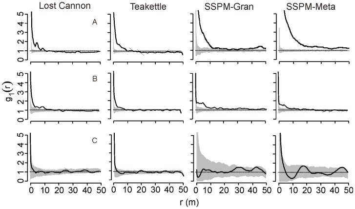
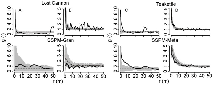
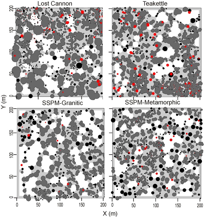
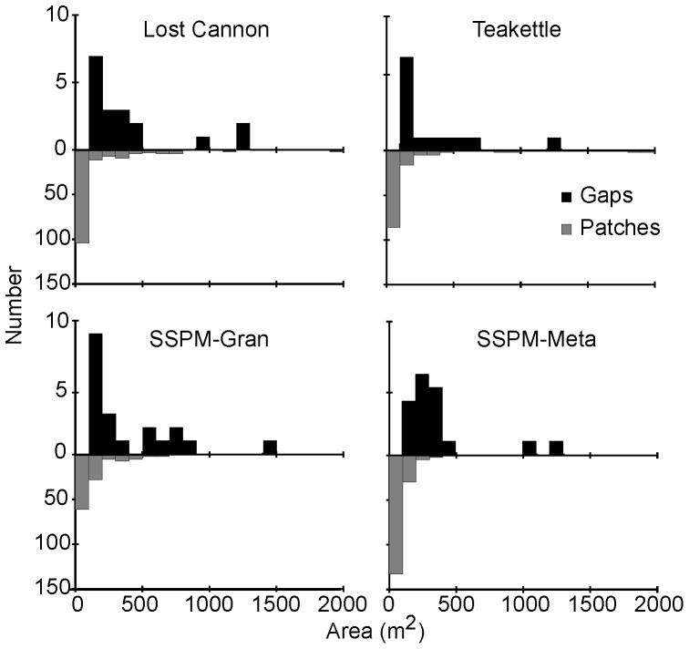
In Mediterranean environments in western North America, historic fire regimes in frequent-fire conifer forests are highly variable both temporally and spatially. This complexity influenced forest structure and spatial patterns, but some of this diversity has been lost due to anthropogenic disruption of ecosystem processes, including fire. Information from reference forest sites can help management efforts to restore forests conditions that may be more resilient to future changes in disturbance regimes and climate. In this study, we characterize tree spatial patterns using four-ha stem maps from four old-growth, Jeffrey pine-mixed conifer forests, two with active-fire regimes in northwestern Mexico and two that experienced fire exclusion in the southern Sierra Nevada. Most of the trees were in patches, averaging six to 11 trees per patch at 0.007 to 0.014 ha(-1), and occupied 27-46% of the study areas. Average canopy gap sizes (0.04 ha) covering 11-20% of the area were not significantly different among sites. The putative main effects of fire exclusion were higher densities of single trees in smaller size classes, larger proportion of trees (≥ 56%) in large patches (≥ 10 trees), and decreases in spatial complexity. While a homogenization of forest structure has been a typical result from fire exclusion, some similarities in patch, single tree, and gap attributes were maintained at these sites. These within-stand descriptions provide spatially relevant benchmarks from which to manage for structural heterogeneity in frequent-fire forest types.
Overview
The claims and statistics of this paper haven’t been checked yet.
Free: it reads the open-access text and checks the first 5 claims that cite a source we can check. Create a free account to check every claim.
Integrity signals
Registry
Cites
Statistics
Figures







Verification
Claims the paper makes
The claims and statistics of this paper haven’t been checked yet.
Free: it reads the open-access text and checks the first 5 claims that cite a source we can check. Create a free account to check every claim.
Self-check
Percentages, sums and reported differences re-computed from the paper’s own numbers.
The self-check needs the paper’s full text.
Citations
Cites
Warming and earlier spring increase western U.S. forest wildfire activity.
Westerling, A. L., Hidalgo, H. G., Cayan, D. R., & Swetnam, T. W. (2006) · Science · doi:10.1126/science.1128834 · Cited by 5,176
Bowman, D. M. J. S., Balch, J. K., Artaxo, P., Bond, W. J., Carlson, J. M., Cochrane, M. A., D’Antonio, C. M., DeFries, R. S., Doyle, J. C., Harrison, S. P., et al. (2009) · Science · doi:10.1126/science.1163886 · Cited by 3,351
spatstat: An R Package for Analyzing Spatial Point Patterns
Baddeley, A., & Turner, R. (2005) · Journal of Statistical Software · doi:10.18637/jss.v012.i06 · Cited by 2,328
CLIMATE CHANGE AND FORESTS OF THE FUTURE: MANAGING IN THE FACE OF UNCERTAINTY
Millar, C. I., Stephenson, N. L., & Stephens, S. L. (2007) · Ecological Applications · doi:10.1890/06-1715.1 · Cited by 2,006
Self-citationFranklin, J. F., Spies, T. A., Pelt, R. V., Carey, A. B., Thornburgh, D. A., Berg, D. R., Lindenmayer, D. B., Harmon, M. E., Keeton, W. S., Shaw, D. C., et al. (2002) · Forest Ecology and Management · doi:10.1016/s0378-1127(01)00575-8 · Cited by 1,791
Multivariate Statistics for Wildlife and Ecology Research
McGarigal, K., Stafford, S., & Cushman, S. (2000) · doi:10.1007/978-1-4612-1288-1 · Cited by 1,548
Rings, circles and null models for point pattern analysis in ecology.
Wiegand, T., & A. Moloney, K. (2004) · Oikos · doi:10.1111/j.0030-1299.2004.12497.x · Cited by 1,157
Gasith, A., & Resh, V. H. (1999) · Annual Review of Ecology and Systematics · doi:10.1146/annurev.ecolsys.30.1.51 · Cited by 1,104
Landscape—wildfire interactions in southern Europe: implications for landscape management
Moreira, F., Viedma, O., Arianoutsou, M., Curt, T., Koutsias, N., Rigolot, E., Barbati, A., Corona, P., Vaz, P., Xanthopoulos, G., et al. (2011) · Journal of Environmental Management · doi:10.1016/j.jenvman.2011.06.028 · Cited by 926
Are wildfires a disaster in the Mediterranean basin? – A review
Pausas, J. G., Llovet, J., Rodrigo, A., & Vallejo, R. (2008) · International Journal of Wildland Fire · doi:10.1071/wf07151 · Cited by 843
Research works printed but not linked: 2
- Zar JH (1999) Biostatistical analysis. Fourth edition. New Jersey: Prentice Hall.
- North M, Sherlock J (2012) Marking and assessing forest heterogeneity. In: North M, Ed. Managing Sierra Nevada Forests. USDA Forest Service General Technical Report PSW-237. Pacific Southwest Research Station, Albany, California. · DOI · Paper page
Cited by
Drought, Tree Mortality, and Wildfire in Forests Adapted to Frequent Fire
Stephens, S. L., Collins, B. M., Fettig, C. J., Finney, M. A., Hoffman, C. M., Knapp, E. E., North, M. P., Safford, H., & Wayman, R. B. (2018) · BioScience · doi:10.1093/biosci/bix146 · Cited by 407
Self-citationHagmann, R. K., Hessburg, P. F., Prichard, S. J., Povak, N. A., Brown, P. M., Fulé, P. Z., Keane, R. E., Knapp, E. E., Lydersen, J. M., Metlen, K. L., et al. (2021) · Ecological Applications · doi:10.1002/eap.2431 · Cited by 400
“…very fine spatial scales (<1 ha) resulting in a mosaic of individual trees, clumps of trees, and openings, rather than patches or stands (Franklin and Van Pelt 2004, Kaufmann et al. 2007, Larson and Churchill 2012, Churchill et al. 2013, 2017, Lydersen et al. 2013, Fry et al. 2014, Ng et al. 2020).”
BackgroundSelf-citationTowards a comprehensive look at global drivers of novel extreme wildfire events
Duane, A., Castellnou, M., & Brotons, L. (2021) · Climatic Change · doi:10.1007/s10584-021-03066-4 · Cited by 329
Climate, Environment, and Disturbance History Govern Resilience of Western North American Forests
Hessburg, P. F., Miller, C. L., Parks, S. A., Povak, N. A., Taylor, A. H., Higuera, P. E., Prichard, S. J., North, M. P., Collins, B. M., Hurteau, M. D., et al. (2019) · Frontiers in Ecology and Evolution · doi:10.3389/fevo.2019.00239 · Cited by 308
Self-citationRestoring fire-prone Inland Pacific landscapes: seven core principles
Hessburg, P. F., Churchill, D. J., Larson, A. J., Haugo, R. D., Miller, C., Spies, T. A., North, M. P., Povak, N. A., Belote, R. T., Singleton, P. H., et al. (2015) · Landscape Ecology · doi:10.1007/s10980-015-0218-0 · Cited by 280
Self-citation
Metadata
- Authors
- Fry, D. L., Stephens, S. L., Collins, B. M., North, M. P., Franco-Vizcaíno, E., & Gill, S. J.
- Affiliations
- University of California, Berkeley (US)
- US Forest Service (US)
- California Polytechnic State University (US)
- Corresponding author
- Fry, Danny L.
- Venue
- PLoS ONE
- Publisher
- Public Library of Science (PLoS)
- Published
- 2014-02-20
- Volume
- 9
- Issue
- 2
- Pages
- e88985
- ISSN
- 1932-6203 (ISSN-L)
- PMC
- PMC3930671
- OpenAlex
- W2045205570
- Cited by
- 61
- References
- 114
- Citations by year
- 2026: 2 · 2025: 2 · 2024: 5 · 2023: 4 · 2022: 4 · 2021: 5 · 2020: 8 · 2019: 3 · 2018: 6 · 2017: 5 · 2016: 7 · 2015: 8 · 2014: 2
- FWCI
- 6.02
- Type
- journal article
- Language
- en
- Open access
- gold
- doi.org
- Licence
- Locations
- PLoS ONE (publishedVersion, public-domain)
- Europe PMC (PubMed Central) (publishedVersion, public-domain)
- PubMed Central (publishedVersion, public-domain)
- PubMed (publishedVersion)
- DOAJ (DOAJ: Directory of Open Access Journals) (submittedVersion)
- eScholarship (California Digital Library) (submittedVersion)
- Figshare (submittedVersion, cc-by)
- Funders
- U.S. Department of Agriculture
- Topics
- Physical Sciences › Environmental Science › Global and Planetary Change › Fire effects on ecosystems
- Life Sciences › Agricultural and Biological Sciences › Forestry › Forest ecology and management
- Physical Sciences › Environmental Science › Nature and Landscape Conservation › Ecology and Vegetation Dynamics Studies
- Keywords
- tree spatial patterns, fire suppression, old-growth forest, Jeffrey pine, mixed conifer forest, canopy gaps, patch size, structural heterogeneity, forest restoration, Sierra Nevada, northwestern Mexico
- MeSH terms
- California, Climate, Demography, Fires, Mexico, Population Density, Species Specificity, Forestry, Tracheophyta, Forests
About these checks
Registry, retraction, Cites and statistics results are computed, not judged, with one exception: a printed reference that no index lists is read once by a model before it counts as a citation error. Claims are extracted by a model and kept only when their quote appears verbatim in the text; each cited source is then checked, with a model’s help, for whether it says what the claim relies on. Those verdicts can be wrong — read the claim’s quote and the cited source before relying on one.
Statistics and arithmetic are recomputed, not judged.
Confidence bands are shown only for fields calibrated on our annotated test set. None is calibrated yet, so no band is shown.
What counts as a claim ›How we measure confidence ›How we check this ›
Are you an author, or do you see a problem with this page? Request a review
How to cite
Cite CoChat for the checks on this page, and the paper for its own findings.
- This page
- CoChat. (2026). Citation check: Contrasting Spatial Patterns in Active-Fire and Fire-Suppressed Mediterranean Climate Old-Growth Mixed Conifer Forests. https://app.cochat.ai/papers/10.1371/journal.pone.0088985
- The paper
- Fry, D. L., Stephens, S. L., Collins, B. M., North, M. P., Franco-Vizcaíno, E., & Gill, S. J. (2014). Contrasting Spatial Patterns in Active-Fire and Fire-Suppressed Mediterranean Climate Old-Growth Mixed Conifer Forests. PLoS ONE. https://doi.org/10.1371/journal.pone.0088985
Data sources
Bibliographic data: Semantic Scholar, OpenAlex, Crossref.
Contains information from the Semantic Scholar Academic Graph Datasets, made available under the ODC Attribution License (ODC-BY 1.0).
Semantic Scholar’s data is described in: Kinney, R., et al. (2023). The Semantic Scholar Open Data Platform. arXiv:2301.10140.
