

The DOI matches its Crossref record; 94 of the 96 references it cites were found in a registry or an index.
Comparing and evaluating metagenome assembly tools from a microbiologist's perspective - not only size matters!
Open accessAbstract
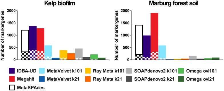
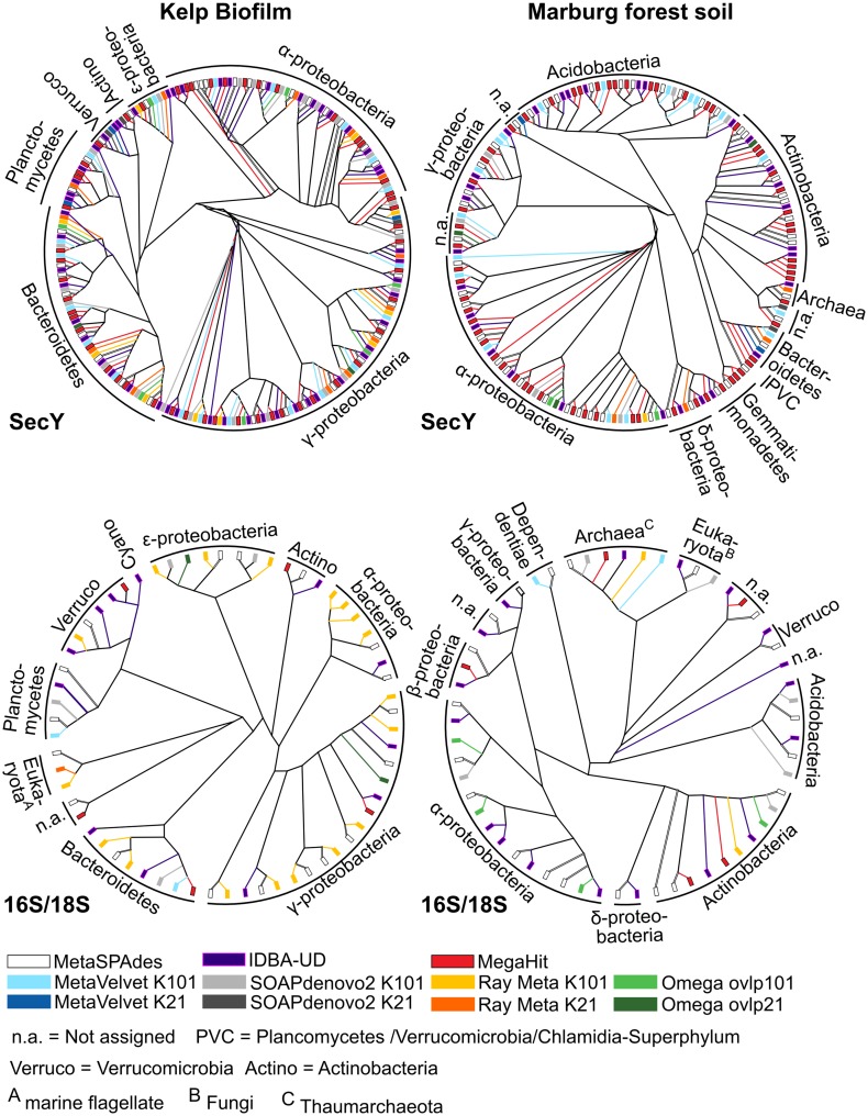
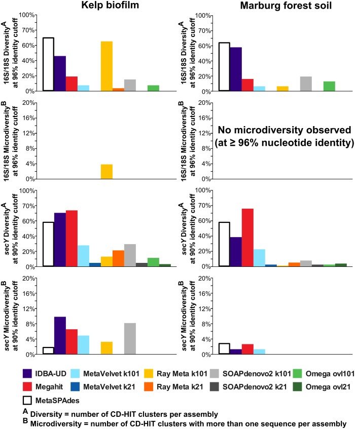
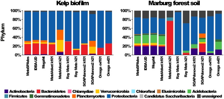
With the constant improvement in cost-efficiency and quality of Next Generation Sequencing technologies, shotgun-sequencing approaches -such as metagenomics- have nowadays become the methods of choice for studying and classifying microorganisms from various habitats. The production of data has dramatically increased over the past years and processing and analysis steps are becoming more and more of a bottleneck. Limiting factors are partly the availability of computational resources, but mainly the bioinformatics expertise in establishing and applying appropriate processing and analysis pipelines. Fortunately, a large diversity of specialized software tools is nowadays available. Nevertheless, choosing the most appropriate methods for answering specific biological questions can be rather challenging, especially for non-bioinformaticians. In order to provide a comprehensive overview and guide for the microbiological scientific community, we assessed the most common and freely available metagenome assembly tools with respect to their output statistics, their sensitivity for low abundant community members and variability in resulting community profiles as well as their ease-of-use. In contrast to the highly anticipated "Critical Assessment of Metagenomic Interpretation" (CAMI) challenge, which uses general mock community-based assembler comparison we here tested assemblers on real Illumina metagenome sequencing data from natural communities of varying complexity sampled from forest soil and algal biofilms. Our observations clearly demonstrate that different assembly tools can prove optimal, depending on the sample type, available computational resources and, most importantly, the specific research goal. In addition, we present detailed descriptions of the underlying principles and pitfalls of publically available assembly tools from a microbiologist's perspective, and provide guidance regarding the user-friendliness, sensitivity and reliability of the resulting phylogenetic profiles.
Overview
The claims and statistics of this paper haven’t been checked yet.
Run the check — free, no account needed. It reads the open-access text and checks the sources it cites.
Integrity signals
Registry
Cites
Statistics
Figures
Verification
Claims the paper makes
The claims and statistics of this paper haven’t been checked yet.
Run the check — free, no account needed. It reads the open-access text and checks the sources it cites.
Claims other papers make about this one
Each is checked against this paper’s own text: does it say what the citing paper says it does?
In the citing paper
“Assembly is a computationally expensive process, frequently requiring terabytes of memory to accomplish when using metaSPAdes (20), which is our primary assembly algorithm, as the ensuing assemblies are typically of better quality than those produced using other assemblers (21).”
From MGnify: the microbiome analysis resource in 2020 (2019) · cites this paper as [21]
Self-check
Percentages, sums and reported differences re-computed from the paper’s own numbers.
The self-check needs the paper’s full text.
Citations
Cites
Trimmomatic: a flexible trimmer for Illumina sequence data
Bolger, A. M., Lohse, M., & Usadel, B. (2014) · Bioinformatics · doi:10.1093/bioinformatics/btu170 · Cited by 65,548
MUSCLE: multiple sequence alignment with high accuracy and high throughput
Edgar, R. C. (2004) · Nucleic Acids Research · doi:10.1093/nar/gkh340 · Cited by 44,662
SPAdes: A New Genome Assembly Algorithm and Its Applications to Single-Cell Sequencing
Bankevich, A., Nurk, S., Antipov, D., Gurevich, A. A., Dvorkin, M. V., Kulikov, A. S., Lesin, V. M., Nikolenko, S., Pham, S., Prjibelski, A. D., et al. (2012) · Journal of Computational Biology · doi:10.1089/cmb.2012.0021 · Cited by 26,312
BLAST+: architecture and applications
Camacho, C., Coulouris, G., Avagyan, V., Ma, N., Papadopoulos, J., Bealer, K., & Madden, T. L. (2009) · BMC Bioinformatics · doi:10.1186/1471-2105-10-421 · Cited by 22,074
FLASH: fast length adjustment of short reads to improve genome assemblies
Magoč, T., & Salzberg, S. L. (2011) · Bioinformatics · doi:10.1093/bioinformatics/btr507 · Cited by 15,366
Fast and sensitive protein alignment using DIAMOND
Buchfink, B., Xie, C., & Huson, D. H. (2015) · Nature Methods · doi:10.1038/nmeth.3176 · Cited by 14,201
Prodigal: prokaryotic gene recognition and translation initiation site identification
Hyatt, D., Chen, G.-L., LoCascio, P. F., Land, M., Larimer, F. W., & Hauser, L. (2010) · BMC Bioinformatics · doi:10.1186/1471-2105-11-119 · Cited by 12,692
Cd-hit: Accelerated for clustering the next-generation sequencing data
Fu, L., Niu, B., Zhu, Z., Wu, S., & Li, W. (2012) · Bioinformatics · doi:10.1093/bioinformatics/bts565 · Cited by 11,175
Li, D., Liu, C.-M., Luo, R., Sadakane, K., & Lam, T. (2015) · Bioinformatics · doi:10.1093/bioinformatics/btv033 · Cited by 10,133
Velvet: Algorithms for de novo short read assembly using de Bruijn graphsPreprint
Zerbino, D. R., & Birney, E. (2008) · Genome Research · doi:10.1101/gr.074492.107 · Cited by 9,587
Sequencing technologies – the next generation
Metzker, M. L. (2010) · Nature Reviews Genetics · doi:10.1038/nrg2626 · Cited by 7,066
ARB: a software environment for sequence data
Ludwig, W. (2004) · Nucleic Acids Research · doi:10.1093/nar/gkh293 · Cited by 6,714
RNAmmer: consistent and rapid annotation of ribosomal RNA genes
Lagesen, K., Hallin, P., Rødland, E., Stærfeldt, H., Rognes, T., & Ussery, D. (2007) · Nucleic Acids Research · doi:10.1093/nar/gkm160 · Cited by 5,965
SOAPdenovo2: an empirically improved memory-efficient short-read de novo assembler
Luo, R., Liu, B., Xie, Y., Li, Z., Huang, W., Yuan, J., He, G., Chen, Y., Pan, Q., Liu, Y., et al. (2012) · GigaScience · doi:10.1186/2047-217x-1-18 · Cited by 5,365
Quality control and preprocessing of metagenomic datasets
Schmieder, R., & Edwards, R. A. (2011) · Bioinformatics · doi:10.1093/bioinformatics/btr026 · Cited by 5,119
metaSPAdes: a new versatile metagenomic assembler
Nurk, S., Meleshko, D., Korobeynikov, A., & Pevzner, P. A. (2017) · Genome Research · doi:10.1101/gr.213959.116 · Cited by 4,496
Peng, Y., Leung, H. C. M., Yiu, S., & Chin, F. Y. L. (2012) · Bioinformatics · doi:10.1093/bioinformatics/bts174 · Cited by 2,998
SINA: Accurate high-throughput multiple sequence alignment of ribosomal RNA genes
Pruesse, E., Peplies, J., & Glöckner, F. (2012) · Bioinform. · doi:10.1093/bioinformatics/bts252 · Cited by 2,989
De novo assembly of human genomes with massively parallel short read sequencing
Li, R., Zhu, H., Ruan, J., Qian, W., Fang, X., Shi, Z., Li, Y., Li, S., Shan, G., Kristiansen, K., et al. (2010) · Genome Research · doi:10.1101/gr.097261.109 · Cited by 2,926
Binning metagenomic contigs by coverage and composition
Alneberg, J., Bjarnason, B. S., de Bruijn, I., Schirmer, M., Quick, J., Ijaz, U. Z., Lahti, L., Loman, N. J., Andersson, A. F., & Quince, C. (2014) · Nature Methods · doi:10.1038/nmeth.3103 · Cited by 2,815
Yarza, P., Yilmaz, P., Pruesse, E., Glöckner, F. O., Ludwig, W., SCHLEIFER, K. H., Whitman, W. B., Euzéby, J. P., Amann, R., & Rossello-Mora, R. A. (2014) · Nature Reviews Microbiology · doi:10.1038/nrmicro3330 · Cited by 2,651
Insights into the phylogeny and coding potential of microbial dark matter
Rinke, C., Schwientek, P., Sczyrba, A., Ivanova, N. N., Anderson, I. J., Cheng, J.-F., Darling, A., Malfatti, S., Swan, B. K., Gies, E. A., et al. (2013) · Nature · doi:10.1038/nature12352 · Cited by 2,394
Interactive metagenomic visualization in a Web browser
Ondov, B., Bergman, N. H., & Phillippy, A. M. (2011) · BMC Bioinformatics · doi:10.1186/1471-2105-12-385 · Cited by 2,123
Pyrosequencing enumerates and contrasts soil microbial diversity
Roesch, L. F. W., Fulthorpe, R. R., Riva, A., Casella, G., Hadwin, A. K. M., Kent, A. D., Daroub, S. H., Camargo, F. A. D. O., Farmerie, W. G., & Triplett, E. W. (2007) · The ISME Journal · doi:10.1038/ismej.2007.53 · Cited by 1,891
ART: a next-generation sequencing read simulator
Huang, W., Li, L., Myers, J. R., & Marth, G. (2011) · Bioinformatics · doi:10.1093/bioinformatics/btr708 · Cited by 1,548
Degeneracy and complexity in biological systems
Edelman, G. M., & Gally, J. A. (2001) · Proceedings of the National Academy of Sciences · doi:10.1073/pnas.231499798 · Cited by 1,493
Assembling Single-Cell Genomes and Mini-Metagenomes From Chimeric MDA Products
Nurk, S., Bankevich, A., Antipov, D., Gurevich, A. A., Korobeynikov, A., Lapidus, A. L., Prjibelski, A. D., Pyshkin, A., Sirotkin, A., Sirotkin, Y., et al. (2013) · Journal of Computational Biology · doi:10.1089/cmb.2013.0084 · Cited by 1,352
An Eulerian path approach to DNA fragment assembly
Pevzner, P. A., Tang, H., & Waterman, M. S. (2001) · Proceedings of the National Academy of Sciences · doi:10.1073/pnas.171285098 · Cited by 1,352
Albertsen, M., Hugenholtz, P., Skarshewski, A., Nielsen, K. L., Tyson, G. W., & Nielsen, P. H. (2013) · Nature Biotechnology · doi:10.1038/nbt.2579 · Cited by 1,259
Unusual biology across a group comprising more than 15% of domain Bacteria
Brown, C. T., Hug, L. A., Thomas, B. C., Sharon, I., Castelle, C. J., Singh, A., Wilkins, M. J., Wrighton, K. C., Williams, K. H., & Banfield, J. F. (2015) · Nature · doi:10.1038/nature14486 · Cited by 1,216
The Next-Generation Sequencing Revolution and Its Impact on Genomics
Koboldt, D. C., Steinberg, K. M., Larson, D. E., Wilson, R. K., & Mardis, E. R. (2013) · Cell · doi:10.1016/j.cell.2013.09.006 · Cited by 1,098
Baldrián, P., Kolařík, M., Štursová, M., Kopecký, J., Brabcová, V., Větrovský, T., Žifčáková, L., Šnajdr, J., Rídl, J., Vlček, Č., et al. (2011) · The ISME Journal · doi:10.1038/ismej.2011.95 · Cited by 865
Daniel, R. (2005) · Nature Reviews Microbiology · doi:10.1038/nrmicro1160 · Cited by 862
Microbial life under extreme energy limitation
Hoehler, T. M., & Jørgensen, B. B. (2013) · Nature Reviews Microbiology · doi:10.1038/nrmicro2939 · Cited by 784
Metagenomic Analyses: Past and Future Trends
Simon, C., & Daniel, R. (2010) · Applied and Environmental Microbiology · doi:10.1128/aem.02345-10 · Cited by 772
Efficient de novo assembly of large genomes using compressed data structuresPreprint
Simpson, J. T., & Durbin, R. M. (2011) · Genome Research · doi:10.1101/gr.126953.111 · Cited by 767
Wooley, J., Godzik, A., & Friedberg, I. (2010) · PLoS Computational Biology · doi:10.1371/journal.pcbi.1000667 · Cited by 763
Wu, Y., Tang, Y.-H., Tringe, S. G., Simmons, B. A., & Singer, S. W. (2014) · Microbiome · doi:10.1186/2049-2618-2-26 · Cited by 725
DECIPHER, a Search-Based Approach to Chimera Identification for 16S rRNA Sequences
Wright, E. S., Yilmaz, L. S., & Noguera, D. R. (2011) · Applied and Environmental Microbiology · doi:10.1128/aem.06516-11 · Cited by 719
Namiki, T., Hachiya, T., Tanaka, H. L., & Sakakibara, Y. (2012) · Nucleic Acids Research · doi:10.1093/nar/gks678 · Cited by 669
PhyloSift: phylogenetic analysis of genomes and metagenomes
Darling, A. E., Jospin, G., Lowe, E., Matsen, F. A., IV, Bik, H. M., & Eisen, J. A. (2014) · PeerJ · doi:10.7717/peerj.243 · Cited by 625
Ray Meta: scalable de novo metagenome assembly and profiling
Boisvert, S., Raymond, F., Godzaridis, É., Laviolette, F., & Corbeil, J. (2012) · Genome biology · doi:10.1186/gb-2012-13-12-r122 · Cited by 590
Ray: Simultaneous Assembly of Reads from a Mix of High-Throughput Sequencing Technologies
Boisvert, S., Laviolette, F., & Corbeil, J. (2010) · J. Comput. Biol. · doi:10.1089/cmb.2009.0238 · Cited by 563
Albertsen, M., Karst, S. M., Ziegler, A., Kirkegaard, R. H., & Nielsen, P. H. (2015) · PLoS ONE · doi:10.1371/journal.pone.0132783 · Cited by 540
plasmidSPAdes: assembling plasmids from whole genome sequencing data
Antipov, D., Hartwick, N. T., Shen, M. W., Raiko, M., Lapidus, A. L., & Pevzner, P. A. (2016) · Bioinformatics · doi:10.1093/bioinformatics/btw493 · Cited by 539
A first look at the Oxford Nanopore MinION sequencer
Mikheyev, A. S., & Tin, M. M. Y. (2014) · Molecular Ecology Resources · doi:10.1111/1755-0998.12324 · Cited by 483
BayesHammer: Bayesian clustering for error correction in single-cell sequencing
Nikolenko, S., Korobeynikov, A., & Alekseyev, M. A. (2013) · BMC Genomics · doi:10.1186/1471-2164-14-s1-s7 · Cited by 479
An Extensive Evaluation of Read Trimming Effects on Illumina NGS Data Analysis
Fabbro, C. D., Scalabrin, S., Morgante, M., & Giorgi, F. M. (2013) · PLoS ONE · doi:10.1371/journal.pone.0085024 · Cited by 478
Nagarajan, N., & Pop, M. (2013) · Nature Reviews Genetics · doi:10.1038/nrg3367 · Cited by 474
Short read fragment assembly of bacterial genomesPreprint
Chaisson, M., & Pevzner, P. A. (2007) · Genome Research · doi:10.1101/gr.7088808 · Cited by 444
The fragment assembly string graph
Myers, E. W. (2005) · Bioinformatics · doi:10.1093/bioinformatics/bti1114 · Cited by 424
Exploiting sparseness in de novo genome assembly
Ye, C., Ma, Z. S., Cannon, C. H., Pop, M., & Yu, D. W. (2012) · BMC Bioinformatics · doi:10.1186/1471-2105-13-s6-s1 · Cited by 414
Li, D., Liu, C.-M., Luo, R., et al. (2014) · arXiv (Cornell University) · doi:10.48550/arxiv.1409.7208 · Cited by 399
IMG/M: a data management and analysis system for metagenomes
Markowitz, V. M., Ivanova, N., Szeto, E., Palaniappan, K., Chu, K., Dalevi, D., Chen, I.-M. A., Grechkin, Y., Dubchak, I. L., Anderson, I., et al. (2007) · Nucleic Acids Research · doi:10.1093/nar/gkm869 · Cited by 392
The khmer software package: enabling efficient nucleotide sequence analysis
Crusoe, M., Alameldin, H. F., Awad, S., Boucher, E., Caldwell, A., Cartwright, R., Charbonneau, A. L., Constantinides, B., Edvenson, G., Fay, S. A., et al. (2015) · F1000Research · doi:10.12688/f1000research.6924.1 · Cited by 371
Miller, C. S., Baker, B. J., Thomas, B. C., Singer, S. W., & Banfield, J. F. (2011) · Genome biology · doi:10.1186/gb-2011-12-5-r44 · Cited by 347
Meta-IDBA: a de Novo assembler for metagenomic data
Peng, Y., Leung, H. C. M., Yiu, S., & Chin, F. Y. L. (2011) · Bioinformatics · doi:10.1093/bioinformatics/btr216 · Cited by 330
Accurate and universal delineation of prokaryotic species
Mende, D. R., Sunagawa, S., Zeller, G., & Bork, P. (2013) · Nature Methods · doi:10.1038/nmeth.2575 · Cited by 327
Tackling soil diversity with the assembly of large, complex metagenomes
Howe, A. C., Jansson, J. K., Malfatti, S., Tringe, S. G., Tiedje, J. M., & Brown, C. T. (2014) · Proceedings of the National Academy of Sciences · doi:10.1073/pnas.1402564111 · Cited by 322
GroopM: an automated tool for the recovery of population genomes from related metagenomes
Imelfort, M., Parks, D. H., Woodcroft, B. J., Dennis, P. G., Hugenholtz, P., & Tyson, G. W. (2014) · PeerJ · doi:10.7717/peerj.603 · Cited by 315
Using the Metagenomics RAST Server (MG-RAST) for Analyzing Shotgun MetagenomesPreprint
Glass, E. M., Wilkening, J., Wilke, A., Antonopoulos, D. A., & Meyer, F. (2010) · Cold Spring Harbor Protocols · doi:10.1101/pdb.prot5368 · Cited by 304
Li, Z., Chen, Y., Mu, D., Yuan, J., Shi, Y., Zhang, H., Gan, J., Li, N., Hu, X., Liu, B., et al. (2011) · Briefings in Functional Genomics · doi:10.1093/bfgp/elr035 · Cited by 292
Third Generation DNA Sequencing: Pacific Biosciences' Single Molecule Real Time Technology
McCarthy, A. A. (2010) · Chemistry & Biology · doi:10.1016/j.chembiol.2010.07.004 · Cited by 244
Planctomycetes dominate biofilms on surfaces of the kelp Laminaria hyperborea
Bengtsson, M. M., & Øvreås, L. (2010) · BMC Microbiology · doi:10.1186/1471-2180-10-261 · Cited by 241
MetAMOS: a modular and open source metagenomic assembly and analysis pipeline
Treangen, T. J., Koren, S., Sommer, D. D., Liu, B., Astrovskaya, I., Ondov, B., Darling, A. E., Phillippy, A. M., & Pop, M. (2013) · Genome biology · doi:10.1186/gb-2013-14-1-r2 · Cited by 232
Structure, fluctuation and magnitude of a natural grassland soil metagenome
Delmont, T. O., Prestat, E., Keegan, K. P., Faubladier, M., Robe, P., Clark, I. M., Pelletier, É., Hirsch, P. R., Meyer, F., Gilbert, J. A., et al. (2012) · The ISME Journal · doi:10.1038/ismej.2011.197 · Cited by 217
Microbial Community Analysis Using MEGAN
Huson, D. H., & Weber, N. (2013) · Methods in enzymology on CD-ROM/Methods in enzymology · doi:10.1016/b978-0-12-407863-5.00021-6 · Cited by 213
McCoy, R. C., Taylor, R. W., Blauwkamp, T. A., Kelley, J. L., Kertesz, M., Pushkarev, D., Petrov, D. A., & Fiston-Lavier, A.-S. (2014) · PLoS ONE · doi:10.1371/journal.pone.0106689 · Cited by 206
MOCAT: A Metagenomics Assembly and Gene Prediction Toolkit
Kultima, J. R., Sunagawa, S., Li, J., Chen, W., Chen, H., Mende, D. R., Arumugam, M., Pan, Q., Liu, B., Qin, J., et al. (2012) · PLoS ONE · doi:10.1371/journal.pone.0047656 · Cited by 204
Seasonal dynamics of bacterial biofilms on the kelp Laminaria hyperborea
Bengtsson, M. M., Sjøtun, K., & Øvreås, L. (2010) · Aquatic Microbial Ecology · doi:10.3354/ame01409 · Cited by 174
Multi -omics and metabolic modelling pipelines: Challenges and tools for systems microbiology
Fondi, M., & Lió, P. (2015) · Microbiological Research · doi:10.1016/j.micres.2015.01.003 · Cited by 173
Bürgmann, H., Widmer, F., Sigler, W. V., & Zeyer, J. (2003) · Applied and Environmental Microbiology · doi:10.1128/aem.69.4.1928-1935.2003 · Cited by 165
Reconstructing 16S rRNA genes in metagenomic data
Yuan, C., Lei, J., Cole, J. R., & Sun, Y. (2015) · Bioinformatics · doi:10.1093/bioinformatics/btv231 · Cited by 156
Detection of low-abundance bacterial strains in metagenomic datasets by eigengenome partitioning
Cleary, B., Brito, I., Huang, K. H., Gevers, D., Shea, T., Young, S., & Alm, E. J. (2015) · Nature Biotechnology · doi:10.1038/nbt.3329 · Cited by 150
Wang, Y., Leung, H. C. M., Yiu, S., & Chin, F. Y. L. (2012) · Bioinformatics · doi:10.1093/bioinformatics/bts397 · Cited by 144
Terrat, S., Christen, R., Dequiedt, S., Lelièvre, M., Nowak, V., Régnier, T., Bachar, D., Plassart, P., Wincker, P., Jolivet, C., et al. (2011) · Microbial Biotechnology · doi:10.1111/j.1751-7915.2011.00307.x · Cited by 135
The Potential of Metagenomic Approaches for Understanding Soil Microbial Processes
Myrold, D. D., Zeglin, L. H., & Jansson, J. K. (2013) · Soil Science Society of America Journal · doi:10.2136/sssaj2013.07.0287dgs · Cited by 125
Woebken, D., Teeling, H., Wecker, P., Dumitriu, A., Kostadinov, I., DeLong, E. F., Amann, R., & Glöckner, F. O. (2007) · The ISME Journal · doi:10.1038/ismej.2007.63 · Cited by 122
Ghai, R., Martín-Cuadrado, A.-B., Gonzaga, A., García-Heredia, I., Cabrera‐Rubio, R., Martín, J. E.-S., Verdú, M., Deschamps, P., Moreira, D., López‐García, P., et al. (2010) · The ISME Journal · doi:10.1038/ismej.2010.44 · Cited by 121
Nucleic acids in the environment
Trevors, J. T. (1996) · Current Opinion in Biotechnology · doi:10.1016/s0958-1669(96)80040-1 · Cited by 120
Afiahayati, Sato, K., & Sakakibara, Y. (2014) · DNA Research · doi:10.1093/dnares/dsu041 · Cited by 118
Omega: an Overlap-graphde novoAssembler for Metagenomics
Haider, B., Ahn, T.-H., Bushnell, B., Chai, J., Copeland, A., & Pan, C. (2014) · Bioinformatics · doi:10.1093/bioinformatics/btu395 · Cited by 96
The Ecology of Microbial Communities Associated with Macrocystis pyrifera
Michelou, V. K., Caporaso, J. G., Knight, R. D., & Palumbi, S. R. (2013) · PLoS ONE · doi:10.1371/journal.pone.0067480 · Cited by 89
Kaster, A., Mayer-Blackwell, K., Passarelli, B., & Spormann, A. M. (2014) · The ISME Journal · doi:10.1038/ismej.2014.24 · Cited by 80
Methanogenic capabilities of ANME-archaea deduced from (13) C-labelling approaches.
Bertram, S., Blumenberg, M., Michaelis, W., Siegert, M., Krüger, M., & Seifert, R. (2013) · Environmental Microbiology · doi:10.1111/1462-2920.12112 · Cited by 74
dipSPAdes: Assembler for Highly Polymorphic Diploid Genomes
Safonova, Y., Bankevich, A., & Pevzner, P. A. (2015) · Journal of Computational Biology · doi:10.1089/cmb.2014.0153 · Cited by 70
Selvaraju, G. D., Fathima, A. A., Radha, S., Arunraj, R., Curtis, W. R., & Ramya, M. (2015) · PLoS ONE · doi:10.1371/journal.pone.0132441 · Cited by 66
metaSPAdes: a new versatile de novo metagenomics assemblerPreprint
Nurk, S., Meleshko, D., Korobeynikov, A., & Pevzner, P. A. (2016) · arXiv (Cornell University) · doi:10.48550/arxiv.1604.03071 · Cited by 46
TruSPAdes: barcode assembly of TruSeq synthetic long reads
Bankevich, A., & Pevzner, P. A. (2016) · Nature Methods · doi:10.1038/nmeth.3737 · Cited by 41
Correction: The Ecology of Microbial Communities Associated with Macrocystis pyrifera
Michelou, V. K., Caporaso, J. G., Knight, R. D., & Palumbi, S. R. (2013) · PLoS ONE · doi:10.1371/annotation/48e29578-a073-42e7-bca4-2f96a5998374 · Cited by 27
De novo meta-assembly of ultra-deep sequencing data
Mirebrahim, H., Close, T. J., & Lonardi, S. (2015) · Bioinformatics · doi:10.1093/bioinformatics/btv226 · Cited by 27
High-speed microbial community profiling
Haft, D. H., & Tovchigrechko, A. (2012) · Nature Methods · doi:10.1038/nmeth.2080 · Cited by 23
The khmer software package: enabling efficient sequence analysis
Brown, C. T., Crusoe, M. R., Edvenson, G., Fish, J. A., Howe, A., McDonald, E., Nahum, J., Nanlohy, K., Ortiz‐Zuazaga, H., Pell, J., et al. (2014) · Figshare · doi:10.6084/m9.figshare.979190 · Cited by 20
dipSPAdes: Assembler for Highly Polymorphic Diploid Genomes
Safonova, Y., Bankevich, A., & Pevzner, P. A. (2014) · Lecture notes in computer science · doi:10.1007/978-3-319-05269-4_21 · Cited by 7
Research works printed but not linked: 2
- B Haider, 2014, Omega: an Overlap-graph de novo Assembler for Metagenomics, Bioinformatics
- L Fu, 2012, CD-HIT: accelerated for clustering the next-generation sequencing data, Bioinformatics
Cited by
Sorted by citations
Microbiome definition re-visited: old concepts and new challenges
Berg, G., Rybakova, D., Fischer, D., Cernava, T., Vergès, M.-C. C., Charles, T., Chen, X., Cocolin, L., Eversole, K., Corral, G. H., et al. (2020) · Microbiome · doi:10.1186/s40168-020-00875-0 · Cited by 2,275
Best practices for analysing microbiomes
Knight, R., Vrbanac, A., Taylor, B. C., Aksenov, A., Callewaert, C., Debelius, J., Gonzalez, A., Kosciolek, T., McCall, L.-I., McDonald, D., et al. (2018) · Nature Reviews Microbiology · doi:10.1038/s41579-018-0029-9 · Cited by 2,030
Allio, R., Schomaker-Bastos, A., Romiguier, J., Prosdocimi, F., Nabholz, B., & Delsuc, F. (2020) · Molecular Ecology Resources · doi:10.1111/1755-0998.13160 · Cited by 1,921
PlasFlow: predicting plasmid sequences in metagenomic data using genome signatures
Krawczyk, P. S., Lipiński, L., & Dziembowski, A. (2017) · Nucleic Acids Research · doi:10.1093/nar/gkx1321 · Cited by 617
Current challenges and best-practice protocols for microbiome analysis
Bharti, R., & Grimm, D. G. (2021) · Briefings in Bioinformatics · doi:10.1093/bib/bbz155 · Cited by 592
Metadata
- Authors
- Vollmers, J., Wiegand, S., & Kaster, A.-K.
- Affiliations
- Leibniz Institute DSMZ – German Collection of Microorganisms and Cell Cultures (DE)
- Corresponding author
- Kaster, Anne-Kristin
- Venue
- PLoS ONE
- Publisher
- Public Library of Science (PLoS)
- Published
- 2017-01-18
- Volume
- 12
- Issue
- 1
- Pages
- e0169662
- ISSN
- 1932-6203 (ISSN-L)
- PMC
- PMC5242441
- OpenAlex
- W2572263783
- Cited by
- 240
- References
- 96
- Citations by year
- 2026: 5 · 2025: 13 · 2024: 28 · 2023: 15 · 2022: 35 · 2021: 37 · 2020: 27 · 2019: 32 · 2018: 25 · 2017: 22
- FWCI
- 11.85
- Type
- journal article
- Language
- en
- Open access
- gold
- doi.org
- Licence
- Locations
- PLoS ONE (publishedVersion, cc-by)
- Europe PMC (PubMed Central) (publishedVersion, cc-by)
- PubMed Central (publishedVersion, cc-by)
- PubMed (publishedVersion)
- DOAJ (DOAJ: Directory of Open Access Journals) (submittedVersion)
- Figshare (submittedVersion, cc-by)
- Funders
- Johns Hopkins University
- University of East Anglia
- Max-Planck-Institut für Terrestrische Mikrobiologie
- Leibniz-Gemeinschaft
- Topics
- Life Sciences › Biochemistry, Genetics and Molecular Biology › Molecular Biology › Genomics and Phylogenetic Studies
- Physical Sciences › Environmental Science › Ecology › Microbial Community Ecology and Physiology
- Physical Sciences › Environmental Science › Ecology › Environmental DNA in Biodiversity Studies
- Keywords
- metagenome assembly, assembler comparison, shotgun sequencing, low-abundance taxa, phylogenetic profiles, algal biofilms, CAMI challenge, mock communities, ease of use
- MeSH terms
- Phylogeny, Software, Soil Microbiology, Macrocystis, Biodiversity, Metagenome, Metagenomics, High-Throughput Nucleotide Sequencing, Forests
About these checks
Registry, retraction, Cites and statistics results are computed, not judged, with one exception: a printed reference that no index lists is read once by a model before it counts as a citation error. Claims are extracted by a model and kept only when their quote appears verbatim in the text; each cited source is then checked, with a model’s help, for whether it says what the claim relies on. Those verdicts can be wrong — read the claim’s quote and the cited source before relying on one.
Statistics and arithmetic are recomputed, not judged.
Confidence bands are shown only for fields calibrated on our annotated test set. None is calibrated yet, so no band is shown.
What counts as a claim ›How we measure confidence ›How we check this ›
Are you an author, or do you see a problem with this page? Request a review
