

The DOI matches its Crossref record; 41 of the 41 references it cites were found in a registry or an index.
A general prediction model for the detection of ADHD and Autism using structural and functional MRI
Open accessAbstract
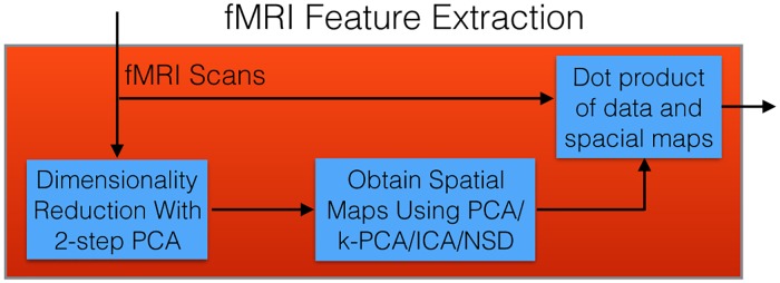
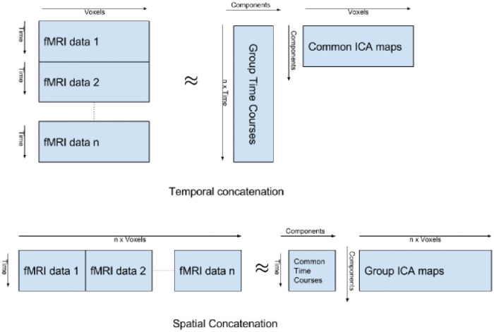
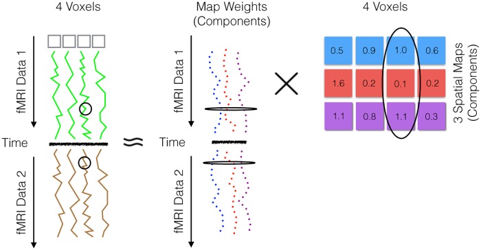
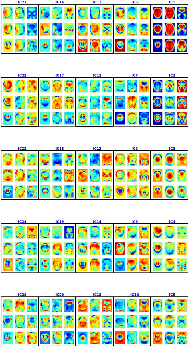
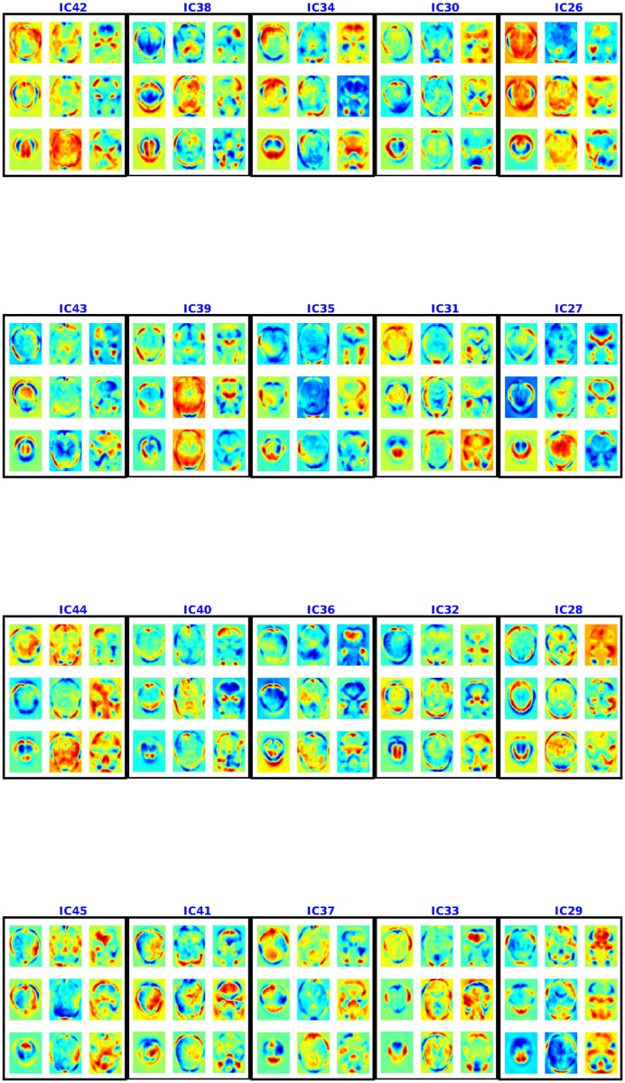
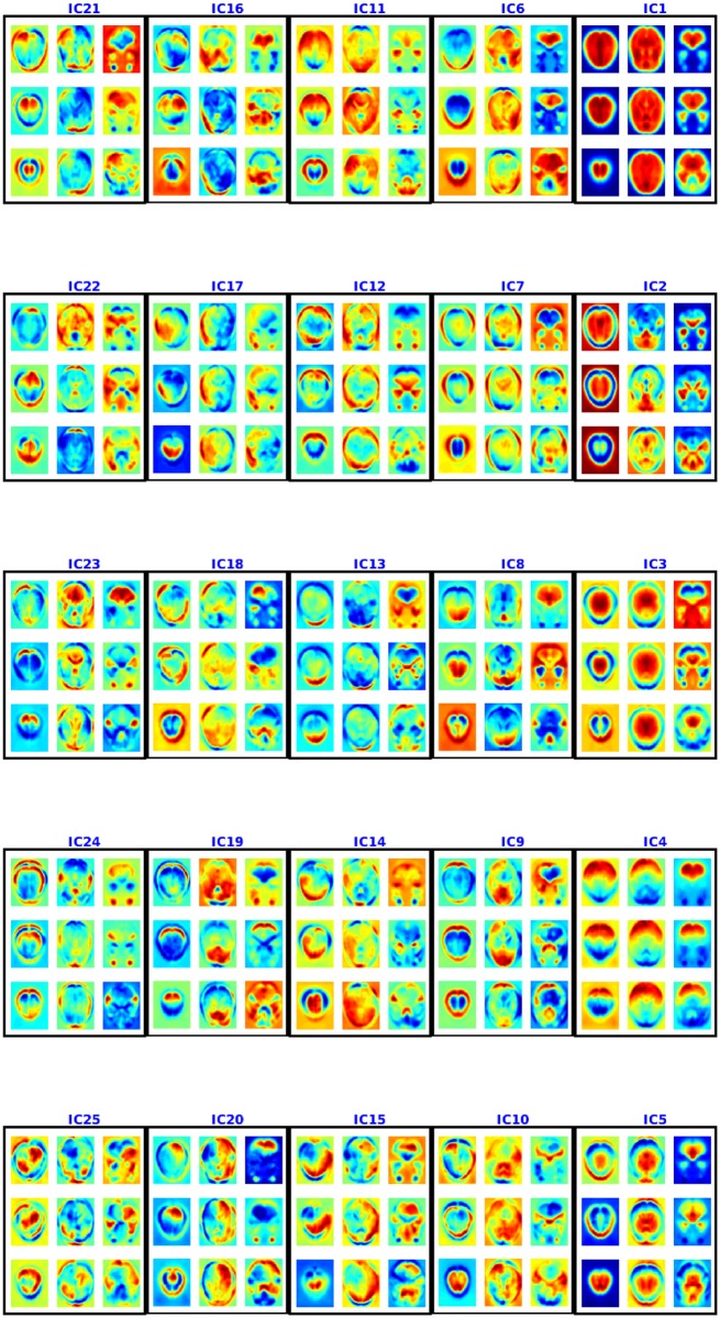
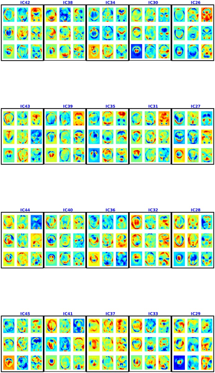
This work presents a novel method for learning a model that can diagnose Attention Deficit Hyperactivity Disorder (ADHD), as well as Autism, using structural texture and functional connectivity features obtained from 3-dimensional structural magnetic resonance imaging (MRI) and 4-dimensional resting-state functional magnetic resonance imaging (fMRI) scans of subjects. We explore a series of three learners: (1) The LeFMS learner first extracts features from the structural MRI images using the texture-based filters produced by a sparse autoencoder. These filters are then convolved with the original MRI image using an unsupervised convolutional network. The resulting features are used as input to a linear support vector machine (SVM) classifier. (2) The LeFMF learner produces a diagnostic model by first computing spatial non-stationary independent components of the fMRI scans, which it uses to decompose each subject's fMRI scan into the time courses of these common spatial components. These features can then be used with a learner by themselves or in combination with other features to produce the model. Regardless of which approach is used, the final set of features are input to a linear support vector machine (SVM) classifier. (3) Finally, the overall LeFMSF learner uses the combined features obtained from the two feature extraction processes in (1) and (2) above as input to an SVM classifier, achieving an accuracy of 0.673 on the ADHD-200 holdout data and 0.643 on the ABIDE holdout data. Both of these results, obtained with the same LeFMSF framework, are the best known, over all hold-out accuracies on these datasets when only using imaging data-exceeding previously-published results by 0.012 for ADHD and 0.042 for Autism. Our results show that combining multi-modal features can yield good classification accuracy for diagnosis of ADHD and Autism, which is an important step towards computer-aided diagnosis of these psychiatric diseases and perhaps others as well.
Overview
The claims and statistics of this paper haven’t been checked yet.
Run the check — free, no account needed. It reads the open-access text and checks the sources it cites.
Integrity signals
Registry
Cites
Statistics
Figures
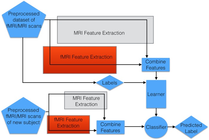
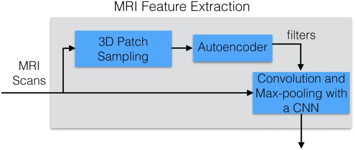
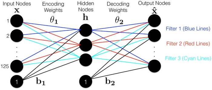
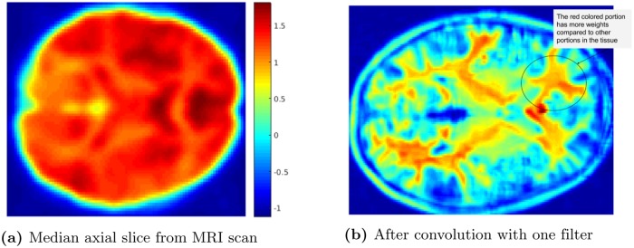

Verification
Claims the paper makes
The claims and statistics of this paper haven’t been checked yet.
Run the check — free, no account needed. It reads the open-access text and checks the sources it cites.
Claims other papers make about this one
Each is checked against this paper’s own text: does it say what the citing paper says it does?
In the citing paper
“A recent study that took advantage of both structural and functional neuroimaging data reported modest, but not clinically useful, accuracy of a complex machine learning algorithm attempting to classify individuals with ASD or ADHD versus TD individuals (Sen et al., 2018).”
From Investigating functional brain network integrity using a traditional and novel categorical scheme for neurodevelopmental disorders (2019) · cites this paper as Sen et al., 2018
In the citing paper
“Biological links such as single nucleotide polymorphisms (4,5), brain structure (6,7), or functional connectivity (8,9) to specific disorders are limited.”
From Methods and challenges for assessing heterogeneity (2020) · cites this paper as [9]
Self-check
Percentages, sums and reported differences re-computed from the paper’s own numbers.
The self-check needs the paper’s full text.
Citations
Cites
Advances in neural information processing systems 7
Cios, K. J., & Shields, M. E. (1997) · Neurocomputing · doi:10.1016/s0925-2312(97)90018-7 · Cited by 22,093
Complex network measures of brain connectivity: Uses and interpretations
Rubinov, M., & Sporns, O. (2010) · NeuroImage · doi:10.1016/j.neuroimage.2009.10.003 · Cited by 11,522
Functional connectivity in the motor cortex of resting human brain using echo‐planar mri
Biswal, B., Zerrin Yetkin, F., Haughton, V. M., & Hyde, J. S. (1995) · Magnetic Resonance in Medicine · doi:10.1002/mrm.1910340409 · Cited by 9,812
Convolutional networks for images, speech, and time series
LeCun, Y., & Bengio, Y. (1998) · HAL · doi:10.5555/303568.303704 · Cited by 4,646
Consistent resting-state networks across healthy subjects
Damoiseaux, J. S., Rombouts, S. A. R. B., Barkhof, F., Scheltens, P., Stam, C. J., Smith, S. M., & Beckmann, C. F. (2006) · Proceedings of the National Academy of Sciences · doi:10.1073/pnas.0601417103 · Cited by 4,326
Methods to detect, characterize, and remove motion artifact in resting state fMRI
Power, J. D., Mitra, A., Laumann, T. O., Snyder, A. Z., Schlaggar, B. L., & Petersen, S. E. (2014) · NeuroImage · doi:10.1016/j.neuroimage.2013.08.048 · Cited by 3,748
A survey of cross-validation procedures for model selectionPreprint
Arlot, S., & Célisse, A. (2009) · Cited by 3,627
A survey of cross-validation procedures for model selection
Arlot, S., & Celisse, A. (2010) · Statistics Surveys · doi:10.1214/09-ss054 · Cited by 3,522
A method for making group inferences from functional MRI data using independent component analysis
Calhoun, V. D., Adali, T., Pearlson, G. D., & Pekar, J. J. (2001) · Human Brain Mapping · doi:10.1002/hbm.1048 · Cited by 2,994
Advances in Neural Information Processing Systems 20
Bonilla, E. V., Chai, K. M. A., & Williams, C. K. I. (2008) · neural information processing systems · Cited by 2,701
Research works printed but not linked: 2
- Ghiassian S, Greiner R, Jin P, Brown M. Learning to classify psychiatric disorders based on fMR images: Autism vs healthy and ADHD vs healthy. In: Proceedings of 3rd NIPS Workshop on Machine Learning and Interpretation in NeuroImaging; 2013.
- Souloumiac A. Blind source detection and separation using second order non-stationarity. In: Acoustics, Speech, and Signal Processing, 1995. ICASSP-95., 1995 International Conference on. vol. 3. IEEE; 1995. p. 1912–1915. · DOI
Cited by
Sorted by citations
The Heterogeneity Problem: Approaches to Identify Psychiatric Subtypes
Feczko, E., Miranda-Dominguez, O., Marr, M., Graham, A. M., Nigg, J. T., & Fair, D. A. (2019) · Trends in Cognitive Sciences · doi:10.1016/j.tics.2019.03.009 · Cited by 443
ASD-DiagNet: A Hybrid Learning Approach for Detection of Autism Spectrum Disorder Using fMRI Data
Eslami, T., Mirjalili, V., Fong, A. C. M., Laird, A. R., & Saeed, F. (2019) · Frontiers in Neuroinformatics · doi:10.3389/fninf.2019.00070 · Cited by 403
“Sen et al. [18] proposed a new algorithm which combines structural and functional features from MRI and fMRI data and got 64 .”
Deep learning in mental health outcome research: a scoping review
Su, C., Xu, Z., Pathak, J., & Wang, F. (2020) · Translational Psychiatry · doi:10.1038/s41398-020-0780-3 · Cited by 368
“One application of DL in fMRI and sMRI data is the identi fi cation of ADHD 25 – 31 .”
BackgroundMethodResultDetection of Autism Spectrum Disorder in Children Using Machine Learning Techniques
Vakadkar, K., Purkayastha, D., & Krishnan, D. (2021) · SN Computer Science · doi:10.1007/s42979-021-00776-5 · Cited by 230
Pagnozzi, A. M., Conti, E., Calderoni, S., Fripp, J., & Rose, S. (2018) · International Journal of Developmental Neuroscience · doi:10.1016/j.ijdevneu.2018.08.010 · Cited by 166
“Indeed, several studies utilise 5-fold (Demirhan, 2018; Sen et al., 2018) and 10-fold cross validation (Akhavan Aghdam et al., 2018; Moradi et al., 2017; Wang et al., 2016).”
Background
Metadata
- Authors
- Sen, B., Borle, N. C., Greiner, R., & Brown, M. R. G.
- Affiliations
- University of Alberta (CA)
- Corresponding author
- Brown, Matthew R. G.
- Venue
- PLOS ONE
- Publisher
- Public Library of Science (PLoS)
- Published
- 2018-04-17
- Volume
- 13
- Issue
- 4
- Pages
- e0194856
- ISSN
- 1932-6203 (ISSN-L)
- PMC
- PMC5903601
- OpenAlex
- W2801745895
- Cited by
- 198
- References
- 41
- Citations by year
- 2026: 9 · 2025: 20 · 2024: 28 · 2023: 25 · 2022: 31 · 2021: 31 · 2020: 36 · 2019: 13 · 2018: 5
- FWCI
- 12.79
- Type
- journal article
- Language
- en
- Open access
- gold
- doi.org
- Licence
- Locations
- PLoS ONE (publishedVersion, cc-by)
- Europe PMC (PubMed Central) (publishedVersion, cc-by)
- PubMed Central (publishedVersion, cc-by)
- PubMed (publishedVersion)
- RePEc: Research Papers in Economics (submittedVersion)
- DOAJ (DOAJ: Directory of Open Access Journals) (submittedVersion)
- Funders
- Canadian Institutes of Health Research (CSE125741)
- Natural Sciences and Engineering Research Council of Canada (NSERC) (203245)
- Alberta Machine Intelligence Institute (AMII)
- Topics
- Life Sciences › Neuroscience › Cognitive Neuroscience › Functional Brain Connectivity Studies
- Health Sciences › Medicine › Psychiatry and Mental health › Attention Deficit Hyperactivity Disorder
- Life Sciences › Neuroscience › Cognitive Neuroscience › Autism Spectrum Disorder Research
- Keywords
- ADHD diagnosis, autism diagnosis, structural MRI, resting-state fMRI, functional connectivity, texture features, sparse autoencoders, independent component analysis, support vector machine, computer-aided diagnosis, multimodal fusion, mental illness
- MeSH terms
- Adolescent, Adult, Attention Deficit Disorder with Hyperactivity, Autistic Disorder, Brain, Child, Decision Support Techniques, Diagnosis, Computer-Assisted, Female, Humans, Image Processing, Computer-Assisted, Magnetic Resonance Imaging, Male, Prognosis, Young Adult, Datasets as Topic
About these checks
Registry, retraction, Cites and statistics results are computed, not judged, with one exception: a printed reference that no index lists is read once by a model before it counts as a citation error. Claims are extracted by a model and kept only when their quote appears verbatim in the text; each cited source is then checked, with a model’s help, for whether it says what the claim relies on. Those verdicts can be wrong — read the claim’s quote and the cited source before relying on one.
Statistics and arithmetic are recomputed, not judged.
Confidence bands are shown only for fields calibrated on our annotated test set. None is calibrated yet, so no band is shown.
What counts as a claim ›How we measure confidence ›How we check this ›
Are you an author, or do you see a problem with this page? Request a review
