

The DOI matches its Crossref record; 196 of the 197 references it cites were found in a registry or an index.
When Null Hypothesis Significance Testing Is Unsuitable for Research: A Reassessment
Open accessPublished version of a preprint
Abstract
Null hypothesis significance testing (NHST) has several shortcomings that are likely contributing factors behind the widely debated replication crisis of (cognitive) neuroscience, psychology, and biomedical science in general. We review these shortcomings and suggest that, after sustained negative experience, NHST should no longer be the default, dominant statistical practice of all biomedical and psychological research. If theoretical predictions are weak we should not rely on all or nothing hypothesis tests. Different inferential methods may be most suitable for different types of research questions. Whenever researchers use NHST they should justify its use, and publish pre-study power calculations and effect sizes, including negative findings. Hypothesis-testing studies should be pre-registered and optimally raw data published. The current statistics lite educational approach for students that has sustained the widespread, spurious use of NHST should be phased out.
Overview
The claims and statistics of this paper haven’t been checked yet.
Run the check — free, no account needed. It reads the open-access text and checks the sources it cites.
Integrity signals
Registry
Cites
Statistics
Figures
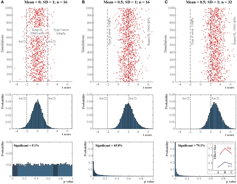
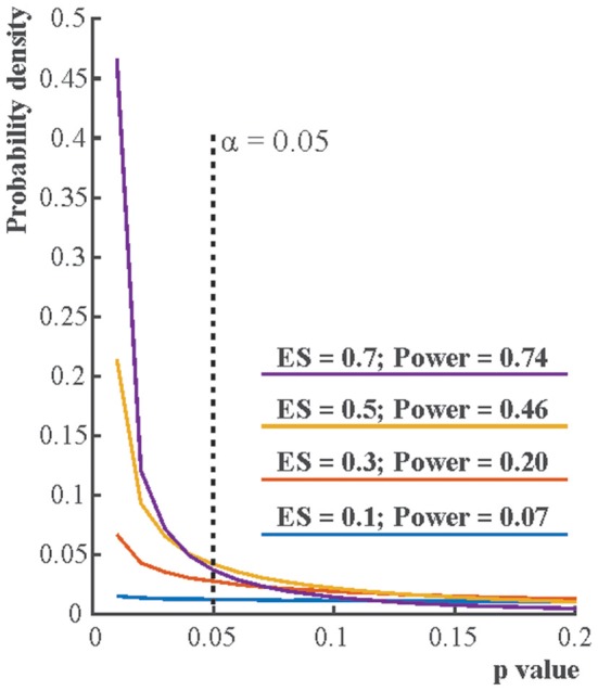
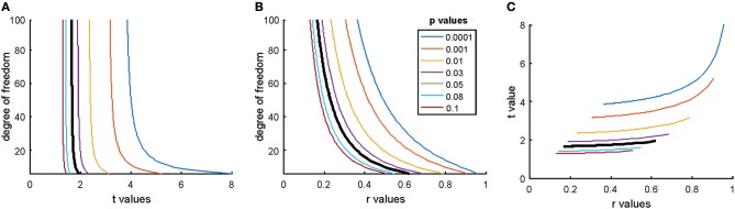
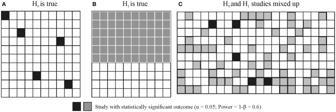
Verification
Claims the paper makes
The claims and statistics of this paper haven’t been checked yet.
Run the check — free, no account needed. It reads the open-access text and checks the sources it cites.
Claims other papers make about this one
Each is checked against this paper’s own text: does it say what the citing paper says it does?
The source backs part of the claim, not all of it — or backs it for a different population, condition or comparison.
In the citing paper
“In cases where complications arise it can be extremely useful to analyse the data with multiple methods to test the robustness of conclusions24,126.”
From A phylogenetic approach to comparative genomics (2025) · cites this paper as [126]
Experimental — accuracy not yet measuredIn the citing paper
“The use of statistical methods has been demonstrated to be suboptimal in some fields.”
From How to design preclinical studies in nanomedicine and cell therapy to maximize the prospects of clinical translation (2018) · cites this paper as [19]
In the citing paper
“Major threats that have high prevalence include the misuse and misinterpretation of null-hypothesis testing methods19,20”
From How to design preclinical studies in nanomedicine and cell therapy to maximize the prospects of clinical translation (2018) · cites this paper as [19]
Self-check
Percentages, sums and reported differences re-computed from the paper’s own numbers.
The self-check needs the paper’s full text.
Citations
Cites
Controlling the False Discovery Rate: A Practical and Powerful Approach to Multiple Testing
Benjamini, Y., & Hochberg, Y. (1995) · Journal of the Royal Statistical Society Series B: Statistical Methodology · doi:10.1111/j.2517-6161.1995.tb02031.x · Cited by 109,482
Gelman, A., Carlin, J. B., Stern, H. S., & Rubin, D. B. (2003) · doi:10.1201/9780429258480 · Cited by 27,276
(1988) · Cited by 16,582
Why Most Published Research Findings Are False
Ioannidis, J. P. A. (2005) · PLoS Medicine · doi:10.1371/journal.pmed.0020124 · Cited by 10,505
Self-citationThe control of the false discovery rate in multiple testing under dependency
Benjamini, Y., & Yekutieli, D. (2001) · The Annals of Statistics · doi:10.1214/aos/1013699998 · Cited by 10,490
Statistical significance for genomewide studies
Storey, J. D., & Tibshirani, R. (2003) · Proceedings of the National Academy of Sciences · doi:10.1073/pnas.1530509100 · Cited by 9,692
Estimating the reproducibility of psychological science
Open Science Collaboration (2015) · Science · doi:10.1126/science.aac4716 · Cited by 8,515 · cited 2×
“, 2014) are in a crisis of producing too many false positive non-replicable results (Begley and Ellis, 2012; Aarts et al., 2015).”
BackgroundStatistical Decision Theory and Bayesian Analysis
Berger, J. O. (1985) · Springer Series in Statistics · doi:10.1007/978-1-4757-4286-2 · Cited by 7,722
Power failure: why small sample size undermines the reliability of neuroscience
Button, K. S., Ioannidis, J. P. A., Mokrysz, C., Nosek, B. A., Flint, J., Robinson, E. S. J., & Munafò, M. R. (2013) · Nature Reviews Neuroscience · doi:10.1038/nrn3475 · Cited by 7,641 · cited 6×
“While power in principle can be adjusted easily by increasing sample size, power in many/most fields of biomedical science and psychology has been notoriously low and the situation has not improved much during the past 50 years (Cohen, 1962; Sedlmeier and Gigerenzer, 1989; Rossi, 1990; Hallahan and Rosenthal, 1996; Bu…”
BackgroundInfluentialSelf-citationSimmons, J. P., Nelson, L. D., & Simonsohn, U. (2011) · Psychological Science · doi:10.1177/0956797611417632 · Cited by 6,567
Research works printed but not linked: 5
- Chaisson, 2017, Astronomy Today
- Cohen, 1988, Statistical Power Analysis for the Behavioural Sciences
- Fisher, 1925, Statistical Methods for Research Workers, First Edition.
- Jeffreys, The Theory of Probability.
- Smolin, 2006, The Trouble with Physics
Cited by
Sorted by citations
Items 201–298 of 298
veRification: an R Shiny application for laboratory method verification and validation
Wilkes, E. H. (2023) · Clinical Chemistry and Laboratory Medicine (CCLM) · doi:10.1515/cclm-2023-0158 · Cited by 3
Siddiqui, N. (2023) · International Journal of Digital Humanities · doi:10.1007/s42803-023-00074-x · Cited by 2
Quantifying error in effect size estimates in attention, executive function, and implicit learning.
Garner, K., Nolan, C. R., Nydam, A. S., Nott, Z. E., Bowman, H., & Dux, P. E. (2024) · Journal of Experimental Psychology Learning Memory and Cognition · doi:10.1037/xlm0001338 · Cited by 2
A Practical Solution to the Multiple-Testing Crisis in Financial ResearchPreprint
de Prado, M. L. (2018) · SSRN Electronic Journal · doi:10.2139/ssrn.3177057 · Cited by 2
Hofmann, A. B., Dörner, M., Machetanz, L., & Kirchebner, J. (2024) · Healthcare · doi:10.3390/healthcare12171699 · Cited by 2
Theoretical models of developmental dyscalculia
Ouyang, X., & Szűcs, D. (2025) · Elsevier eBooks · doi:10.1016/b978-0-443-22224-5.00001-1 · Cited by 1
Ueno, S., & Takeuchi, O. (2025) · Research Methods in Applied Linguistics · doi:10.1016/j.rmal.2025.100256 · Cited by 1
Design and analysis of behavioral intervention studies: A Bayesian approach
Ibáñez, C. N. B., Lösener, U., Moeteke, N. S., & Moerbeek, M. (2026) · PLoS ONE · doi:10.1371/journal.pone.0342163 · Cited by 1
Samples for the Determination of Total 25-Hydroxyvitamin D Levels Were Stable at Ambient Temperature
Wilkes, E. H., Ross, A., & Williams, E. L. (2026) · The Journal of Applied Laboratory Medicine · doi:10.1093/jalm/jfag034 · Cited by 1
Tell me lies, tell me sweet little lies: power calculations in clinical trials
Berk, M., Iyer, R., Mackinnon, A. J., & Cotton, S. (2026) · The British Journal of Psychiatry · doi:10.1192/bjp.2026.10642 · Cited by 1
Piccolo, F., Anderson, E. C., Gutow, H., Johnson, C. M., Nevers, M., DeSanto‐Madeya, S., & Hutchinson, R. N. (2026) · BMC Palliative Care · doi:10.1186/s12904-026-02169-y · Cited by 1
Obtaining Data for Theory Testing: Operationalization, Measurement, and Data Collection
Eisend, M., & Kuß, A. (2019) · Springer eBooks · doi:10.1007/978-3-030-10794-9_6 · Cited by 1
Leeds, A., Riley, A. W., Stalter, L., Terry, M., Alba, A. C., & Soltis, J. M. (2024) · Applied Animal Behaviour Science · doi:10.1016/j.applanim.2024.106338 · Cited by 1
Ramaj, K. (2024) · Bulletin of Sociological Methodology/Bulletin de Méthodologie Sociologique · doi:10.1177/07591063241276753 · Cited by 1
Emprechtinger, R., Schwarzer, G., Schreder, G., Toelch, U., & Gartlehner, G. (2024) · Journal of Clinical Epidemiology · doi:10.1016/j.jclinepi.2024.111640 · Cited by 1
Enhancing Fluency in Speaking through Task-Based Teaching and Learning
Quynh, N. V. (2025) · Journal of Ecohumanism · doi:10.62754/joe.v3i8.5728 · Cited by 2
Proposal for modifying procedures for declaring significant trends in TIMSS
Braun, H. I., von Davier, M., & Chen, J. (2025) · Large-scale Assessments in Education · doi:10.1186/s40536-025-00236-z · Cited by 1
Ioannidis, J. P. A. (2020) · Journal of Clinical Epidemiology · doi:10.1016/j.jclinepi.2020.05.004 · Cited by 1
Self-citationGewinnung von Daten zum Theorietest: Operationalisierung, Messung und Datensammlung
Eisend, M., & Kuß, A. (2021) · Springer eBooks · doi:10.1007/978-3-658-32890-0_6 · Cited by 1
Exploration, inference and prediction in neuroscience and biomedicinePreprint
Bzdok, D., & Ioannidis, J. P. A. (2019) · arXiv (Cornell University) · doi:10.48550/arxiv.1903.10310 · Cited by 1
Self-citationOverview on the Null Hypothesis Significance TestPreprint
van Dongen, N. N. N., & van Grootel, L. (2021) · doi:10.31234/osf.io/hwk4n · Cited by 1
da Costa, G. G. (2021) · doi:10.31219/osf.io/ezmyj · Cited by 1
How do Basic Personality Traits Map onto Moral Judgements of Fairness-related Actions?Preprint
Andrejević, M., Smillie, L. D., Feuerriegel, D., Turner, W., Laham, S. M., & Bode, S. (2020) · PsyArXiv (OSF Preprints) · doi:10.31234/osf.io/e3uxb · Cited by 1
Hirschhorn, R., & Schönberg, T. (2023) · Elsevier eBooks · doi:10.1016/b978-0-12-820480-1.00014-0 · Cited by 1
A critical appraisal of the Dual Process account of moral judgmentPreprint
Quinlan, P. T., & Cohen, D. J. (2023) · doi:10.31234/osf.io/62rgf · Cited by 1
Reproducibility in Preclinical in Vivo Research: Statistical Inferences
Lim, C. J. M., Janhunen, S. K., & Riedel, G. (2024) · Journal of Integrative Neuroscience · doi:10.31083/j.jin2302030 · Cited by 1
Research Integrity in Public Health
Gorman, D. M. (2018) · Oxford University Press eBooks · doi:10.1093/obo/9780199756797-0189
Peña, E. A. (2019) · arXiv (Cornell University) · doi:10.48550/arxiv.1910.05486
Consequences of altering statistical significance threshold in orthopaedic science
Reito, A. R. (2019) · Injury · doi:10.1016/j.injury.2019.11.021
Theory and Approaches in Research into Interaction, Corrective Feedback, and Tasks in L2 Learning
Mackey, A. (2020) · Cambridge University Press eBooks · doi:10.1017/9781108589284.002 · Cited by 1
Mackey, A. (2020) · Cambridge University Press eBooks · doi:10.1017/9781108589284.006
Mackey, A. (2020) · Cambridge University Press eBooks · doi:10.1017/9781108589284.004
Doing Science: Methods and PhilosophyPreprint
van Dongen, N. N. N. (2021) · PsyArXiv (OSF Preprints) · doi:10.31234/osf.io/yegvs
Doing Meta-Analytic and Synthetic Research on Interaction, Feedback, Tasks, and L2 Learning
Mackey, A. (2020) · Cambridge University Press eBooks · doi:10.1017/9781108589284.007
Designing Studies of the Roles of Interaction, Feedback, and Tasks in Second Language Learning
Mackey, A. (2020) · Cambridge University Press eBooks · doi:10.1017/9781108589284.003
Therapeutic Assessment as Preparation for Psychotherapy
Vance, J. M. (2019) · doi:10.12794/metadc1538669
Matematikai pszichológia / pszichológiai statisztika / mérés
Vargha, A. (2022) · Magyar Pszichológiai Szemle · doi:10.1556/0016.2021.00051
Investigating Interaction, Feedback, Tasks, and L2 Learning in Instructional Settings
Mackey, A. (2020) · Cambridge University Press eBooks · doi:10.1017/9781108589284.008
Collecting Introspective Data in Interaction, Feedback, and Task Research
Mackey, A. (2020) · Cambridge University Press eBooks · doi:10.1017/9781108589284.005
Mackey, A. (2020) · Cambridge University Press eBooks · doi:10.1017/9781108589284.011
Mackey, A. (2020) · Cambridge University Press eBooks · doi:10.1017/9781108589284.012
Mackey, A. (2020) · Cambridge University Press eBooks · doi:10.1017/9781108589284.001
Mackey, A. (2020) · Cambridge University Press eBooks · doi:10.1017/9781108589284.013
Mackey, A. (2020) · Cambridge University Press eBooks · doi:10.1017/9781108589284.009
Working with Data in Interaction, Feedback, and Task Research
Mackey, A. (2020) · Cambridge University Press eBooks · doi:10.1017/9781108589284.010
Dissociation Between Speech and Emotion Effects in Short-Term Memory: A Data Reanalysis.
Wiens, S. (2021) · Meta-Psychology · doi:10.15626/mp.2019.1635
Booth, T., Doumas, A., & Murray, A. L. (2020) · Springer eBooks · doi:10.1007/978-3-319-24612-3_1310
Booth, T., Doumas, A., & Murray, A. L. (2017) · Springer eBooks · doi:10.1007/978-3-319-28099-8_1335-1
Booth, T., Doumas, A., & Murray, A. L. (2017) · Springer eBooks · doi:10.1007/978-3-319-28099-8_1310-1
Significance Testing in Natural and Biological Systems: A ReviewPreprint
Kak, S. C. (2021) · doi:10.36227/techrxiv.14599836
Chandran, P. K. G. (2020) · The American Journal of Medicine · doi:10.1016/j.amjmed.2019.12.043
Booth, T., Doumas, A., & Murray, A. L. (2020) · Springer eBooks · doi:10.1007/978-3-319-24612-3_1335
Mackey, A. (2020) · Cambridge University Press eBooks · doi:10.1017/9781108589284.014
Almgren, H., Parsons, N., Bossche, S. V. D., & Marinazzo, D. (2020) · MetArXiv (OSF Preprints) · doi:10.31222/osf.io/9hg3j
Technical and Methodological Comments on McLaughlin et. al. (2018)
Hall, M. E. (2022) · Cliodynamics The Journal of Quantitative History and Cultural Evolution · doi:10.21237/c7clio13054545
Significance Chasing in Hand Surgery Literature
Sankaran, A. (2022) · The Journal of Hand Surgery (Asian-Pacific Volume) · doi:10.1142/s2424835522500643
Cohen’s Convention, the Seriousness of Errors, and the Body of Knowledge in Behavioral SciencePreprint
Arslan, A., & Zenker, F. (2022) · doi:10.31234/osf.io/mjb2x
From Challenges to Opportunities and Open Questions
Mueller, S. (2022) · Springer eBooks · doi:10.1007/978-3-031-18903-6_4
The Challenge of Evaluating Vaccine Safety and Effectiveness
Mueller, S. (2022) · Springer eBooks · doi:10.1007/978-3-031-18903-6_5
Hints of Earlier and Other Creation: Unsupervised Machine Learning in Financial Time-Series Analysis
Chen, J. M., & Agiropoulos, C. (2023) · doi:10.3390/engproc2023039042
Clinical research design and statistics
Tasian, G. E., & Weaver, J. K. (2023) · Elsevier eBooks · doi:10.1016/b978-0-323-77575-5.00042-3
Emmert‐Streib, F., Moutari, S., & Dehmer, M. (2023) · Springer eBooks · doi:10.1007/978-3-031-13339-8_10
The effects of discourse coherence on the persistence of sentence structures.
Zhang, C., Bernolet, S., & Hartsuiker, R. J. (2023) · Journal of Experimental Psychology Learning Memory and Cognition · doi:10.1037/xlm0001295
Gewinnung von Daten zum Theorie-Test: Operationalisierung, Messung und Datensammlung
Eisend, M., & Kuß, A. (2023) · Springer eBooks · doi:10.1007/978-3-658-42690-3_6
Determination of Factors Influencing the Upsurge of Electronic Banking Frauds in Zimbabwe
Manhide, T. C., & Nkomo, D. J. (2023) · Journal of Research and Innovation for Sustainable Society · doi:10.33727/jriss.2023.2.23:189-199
Carlton, J. S., Hartenstine, H., & Shambach, A. M. (2024) · Journal of Risk Research · doi:10.1080/13669877.2024.2437627
Schmaling, K. B., & Kaplan, R. M. (2025) · Cambridge University Press eBooks · doi:10.1017/9781009391733.002
Schmaling, K. B., & Kaplan, R. M. (2025) · Cambridge University Press eBooks · doi:10.1017/9781009391733.007
Schmaling, K. B., & Kaplan, R. M. (2025) · Cambridge University Press eBooks · doi:10.1017/9781009391733.006
Schmaling, K. B., & Kaplan, R. M. (2025) · Cambridge University Press eBooks · doi:10.1017/9781009391733.005
Modeling Soft Skills Development During School-to-Work Programme: A Structural Equation Approach
Graziosi, G., Poliandri, D., & Epifani, G. (2025) · Springer eBooks · doi:10.1007/978-3-031-95995-0_59
Czimbalmos, O., Kőrösi, G., Kékesi, G., & Horvath, G. (2025) · International Convention on Information and Communication Technology, Electronics and Microelectronics · doi:10.1109/mipro65660.2025.11131733
Null Hypothesis Statistical Testing (NHST)
Graham, M. E., & Slaney, K. L. (2025) · Springer eBooks · doi:10.1007/978-3-031-70581-6_9-1
Titensor, S., Ebbert, J. L., Camacho, D., Corte, K. W. D., Palmeira, A. L., Stubbs, R. J., Horgan, G. W., Heitmann, B. L., & Corte, D. D. (2025) · Frontiers in Nutrition · doi:10.3389/fnut.2025.1700898
Meyer, N. (2026) · Journal of Clinical Medicine · doi:10.3390/jcm15062262
The Latina physician wage chasm: a secondary analysis of the American Community Survey
Anaya, Y. B.-M., Hsu, P., Castellon‐Lopez, Y., Pinzon, M. M., Byington, C. L., & Hayes‐Bautista, D. E. (2026) · Academic Medicine · doi:10.1093/acamed/wvag054
Diagnostic et remédiation orientés vers le lexique en compréhension aurale de l'anglais
Jouannaud, M.-P. (2021) · theses.fr (ABES) · doi:10.70675/119e0daaz1bb9z4a45za01bz7613aa8222e7
Evaluating biomarkers and prediction models with E2P SimulatorPreprint
Karvelis, P., Felsky, D., Abi-Dargham, A., Horga, G., & Diaconescu, A. O. (2026) · eLife · doi:10.7554/elife.110646.1
Evaluating biomarkers and prediction models with E2P SimulatorPreprint
Karvelis, P., Felsky, D., Abi-Dargham, A., Horga, G., & Diaconescu, A. O. (2026) · eLife · doi:10.7554/elife.110646
Helman, T. J., Nicholas, M., Lyon, B., Naghipour, S., Kim, C.-K., Ybanez, T., Robertson, K., Griffith, T. A., Peart, J. N., Stapelberg, N. J. C., et al. (2026) · Metabolic Brain Disease · doi:10.1007/s11011-026-01855-3
VRDOLJAK, J. E., Ávila, L. J., Molina, I. S., Benitez‐Vieyra, S., & Morando, M. M. (2026) · Zoological Journal of the Linnean Society · doi:10.1093/zoolinnean/zlag064
Cross-Villasana, F. (2026) · Springer eBooks · doi:10.1007/978-3-032-20450-9_8
The Hypothesis Race Model for evaluation of research findingsPreprint
Kelly, R. E. (2026) · bioRxiv (Cold Spring Harbor Laboratory) · doi:10.64898/2026.05.28.728385
Günver, M. G., Pekerkan, E., Canbaz, M., & Şenocak, M. (2026) · Laboratories · doi:10.3390/laboratories3030014
Bayesian Sample-Size Determination for Longitudinal Trials With Attrition: The BayesSSD Package
Lösener, U., & Moerbeek, M. (2026) · Advances in Methods and Practices in Psychological Science · doi:10.1177/25152459261463494
Settgast, T., Shriki, O., Northoff, G., Zilio, F., Borgheai, S. B., Shahriari, Y., & Kübler, A. (2026) · Research Square · doi:10.21203/rs.3.rs-10422321/v1
Logic of Statistical Inference: Reasoning with E-Values
Hosni, H., & Rad, S. R. (2026) · Journal of Philosophical Logic · doi:10.1007/s10992-026-09862-6
BAYAT, B. (2026) · Research Square · doi:10.21203/rs.3.rs-10632801/v1
Metadata
- Authors
- Szucs, D., & Ioannidis, J. P. A.
- Affiliations
- Stanford Medicine (US)
- Venue
- Frontiers in Human Neuroscience
- Publisher
- Frontiers Media SA
- Published
- 2017-08-03
- Volume
- 11
- Pages
- 390-390
- ISSN
- 1662-5161 (ISSN-L)
- PMC
- PMC5540883
- OpenAlex
- W2951307730
- Cited by
- 298
- References
- 197
- Citations by year
- 2026: 18 · 2025: 28 · 2024: 21 · 2023: 34 · 2022: 44 · 2021: 31 · 2020: 48 · 2019: 39 · 2018: 29 · 2017: 6
- FWCI
- 6.14
- Type
- journal article
- Language
- en
- Open access
- gold
- doi.org
- Licence
- cc-by
- Locations
- Frontiers in Human Neuroscience (publishedVersion, cc-by)
- bioRxiv (Cold Spring Harbor Laboratory) (acceptedVersion, cc-by-nc-nd)
- PubMed Central (publishedVersion, cc-by)
- PubMed (publishedVersion)
- DOAJ (DOAJ: Directory of Open Access Journals) (submittedVersion, cc-by-sa)
- Apollo (University of Cambridge) (submittedVersion, cc-by)
- Apollo (cc-by)
- Funders
- James S. McDonnell Foundation (220020370)
- Topics
- Physical Sciences › Mathematics › Statistics and Probability › Statistical Methods and Bayesian Inference
- Social Sciences › Decision Sciences › Statistics, Probability and Uncertainty › Meta-analysis and systematic reviews
- Physical Sciences › Mathematics › Statistics and Probability › Statistics Education and Methodologies
- Keywords
- null hypothesis significance testing, replication crisis, statistical inference, preregistration, power analysis, effect size, negative results, statistics education, research methodology critique, hypothesis testing
About these checks
Registry, retraction, Cites and statistics results are computed, not judged, with one exception: a printed reference that no index lists is read once by a model before it counts as a citation error. Claims are extracted by a model and kept only when their quote appears verbatim in the text; each cited source is then checked, with a model’s help, for whether it says what the claim relies on. Those verdicts can be wrong — read the claim’s quote and the cited source before relying on one.
Statistics and arithmetic are recomputed, not judged.
Confidence bands are shown only for fields calibrated on our annotated test set. None is calibrated yet, so no band is shown.
What counts as a claim ›How we measure confidence ›How we check this ›
Are you an author, or do you see a problem with this page? Request a review
