

The DOI matches its Crossref record; 58 of the 58 references it cites were found in a registry or an index.
The spatial structure of resting state connectivity stability on the scale of minutes
Open accessAbstract
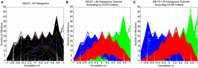
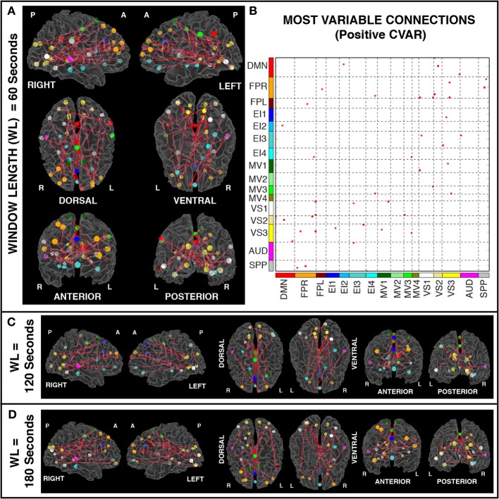
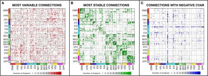
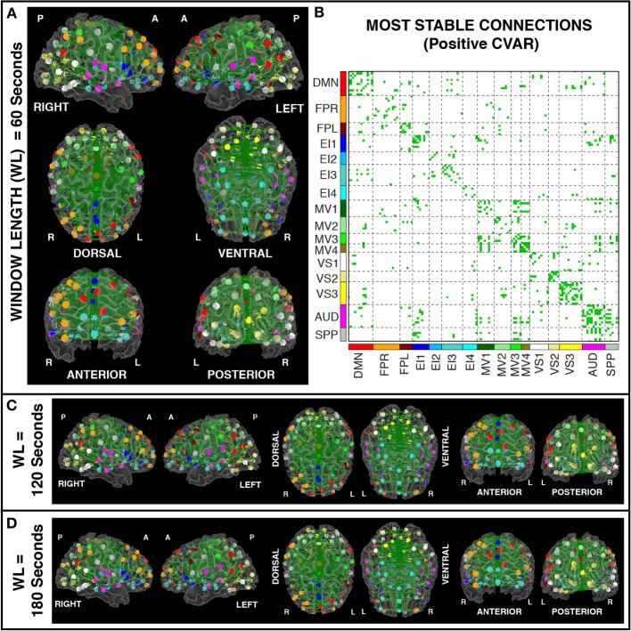
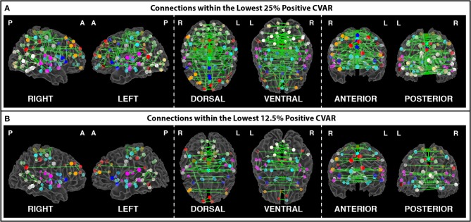
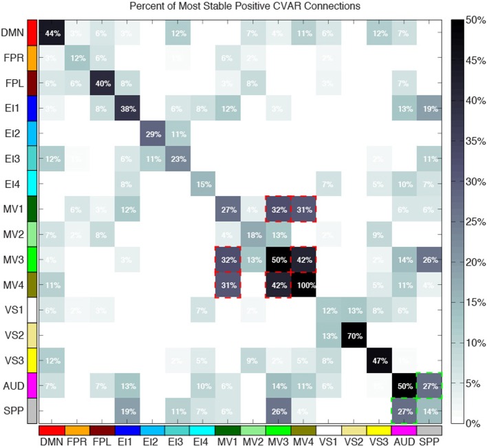
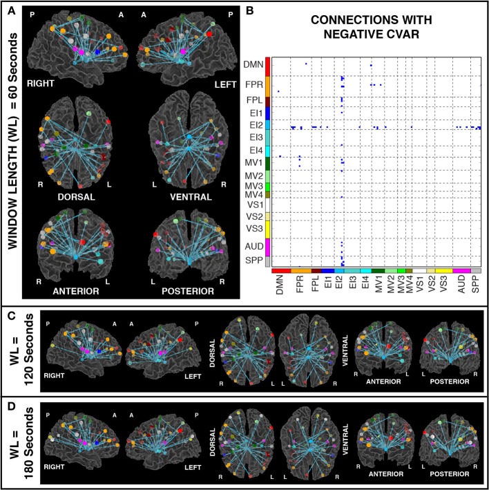
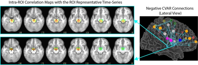
Resting state functional MRI (rsfMRI) connectivity patterns are not temporally stable, but fluctuate in time at scales shorter than most common rest scan durations (5-10 min). Consequently, connectivity patterns for two different portions of the same scan can differ drastically. To better characterize this temporal variability and understand how it is spatially distributed across the brain, we scanned subjects continuously for 60 min, at a temporal resolution of 1 s, while they rested inside the scanner. We then computed connectivity matrices between functionally-defined regions of interest for non-overlapping 1 min windows, and classified connections according to their strength, polarity, and variability. We found that the most stable connections correspond primarily to inter-hemispheric connections between left/right homologous ROIs. However, only 32% of all within-network connections were classified as most stable. This shows that resting state networks have some long-term stability, but confirms the flexible configuration of these networks, particularly those related to higher order cognitive functions. The most variable connections correspond primarily to inter-hemispheric, across-network connections between non-homologous regions in occipital and frontal cortex. Finally we found a series of connections with negative average correlation, but further analyses revealed that such average negative correlations may be related to the removal of CSF signals during pre-processing. Using the same dataset, we also evaluated how similarity of within-subject whole-brain connectivity matrices changes as a function of window duration (used here as a proxy for scan duration). Our results suggest scanning for a minimum of 10 min to optimize within-subject reproducibility of connectivity patterns across the entire brain, rather than a few predefined networks.
Overview
The claims and statistics of this paper haven’t been checked yet.
Run the check — free, no account needed. It reads the open-access text and checks the sources it cites.
Integrity signals
Registry
Cites
Statistics
Figures
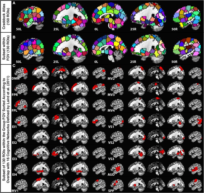
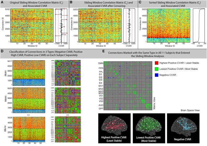
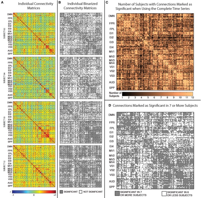
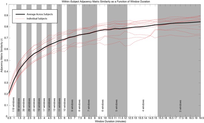
Verification
Claims the paper makes
The claims and statistics of this paper haven’t been checked yet.
Run the check — free, no account needed. It reads the open-access text and checks the sources it cites.
Claims other papers make about this one
Each is checked against this paper’s own text: does it say what the citing paper says it does?
In the citing paper
“Data were then spatially normalized to the Montreal Neurological Institute template using the structural scans; previous studies suggest that this is adequate for reliable functional connectivity estimates 66, 67, 68.”
From History of early life adversity is associated with increased food addiction and sex-specific alterations in reward network connectivity in obesity (2019) · cites this paper as [68]
Self-check
Percentages, sums and reported differences re-computed from the paper’s own numbers.
The self-check needs the paper’s full text.
Citations
Cites
AFNI: Software for analysis and visualization of functional magnetic resonance neuroimages
Cox, R. W. (1996) · Computers and Biomedical Research · doi:10.1006/cbmr.1996.0014 · Cited by 10,913
Functional connectivity in the motor cortex of resting human brain using echo‐planar mri
Biswal, B., Zerrin Yetkin, F., Haughton, V. M., & Hyde, J. S. (1995) · Magnetic Resonance in Medicine · doi:10.1002/mrm.1910340409 · Cited by 9,812
The Brain's Default Network: Anatomy, Function, and Relevance to Disease
Buckner, R. L., Andrews‐Hanna, J. R., & Schacter, D. L. (2008) · Annals of the New York Academy of Sciences · doi:10.1196/annals.1440.011 · Cited by 9,761
The organization of the human cerebral cortex estimated by intrinsic functional connectivity
Thomas Yeo, B. T., Krienen, F. M., Sepulcre, J., Sabuncu, M. R., Lashkari, D., Hollinshead, M., Roffman, J. L., Smoller, J. W., Zöllei, L., Polimeni, J. R., et al. (2011) · Journal of Neurophysiology · doi:10.1152/jn.00338.2011 · Cited by 9,182
Power, J. D., Barnes, K. A., Snyder, A. Z., Schlaggar, B. L., & Petersen, S. E. (2012) · NeuroImage · doi:10.1016/j.neuroimage.2011.10.018 · Cited by 7,429
The organization of the human cerebellum estimated by intrinsic functional connectivity
Buckner, R. L., Krienen, F. M., Castellanos, A., Diaz, J. C., & Yeo, B. T. T. (2011) · Journal of Neurophysiology · doi:10.1152/jn.00339.2011 · Cited by 7,304
Correspondence of the brain's functional architecture during activation and rest
Smith, S. M., Fox, P. T., Miller, K. L., Glahn, D. C., Fox, P. M., Mackay, C. E., Filippini, N., Watkins, K. E., Toro, R., Laird, A. R., et al. (2009) · Proceedings of the National Academy of Sciences · doi:10.1073/pnas.0905267106 · Cited by 5,150
Predicting human resting-state functional connectivity from structural connectivity
Honey, C. J., Sporns, O., Cammoun, L., Gigandet, X., Thiran, J. P., Meuli, R., & Hagmann, P. (2009) · Proceedings of the National Academy of Sciences · doi:10.1073/pnas.0811168106 · Cited by 3,307
Tracking whole-brain connectivity dynamics in the resting state
Allen, E. A., Damaraju, E., Plis, S. M., Erhardt, E. B., Eichele, T., & Calhoun, V. D. (2014) · Cerebral Cortex · doi:10.1093/cercor/bhs352 · Cited by 2,992
Dynamic functional connectivity: Promise, issues, and interpretations
Hutchison, R. M., Womelsdorf, T., Allen, E. A., Bandettini, P. A., Calhoun, V. D., Corbetta, M., Della Penna, S., Duyn, J. H., Glover, G. H., Gonzalez-Castillo, J., et al. (2013) · NeuroImage · doi:10.1016/j.neuroimage.2013.05.079 · Cited by 2,962
Self-citation
Cited by
Sorted by citations
The dynamic functional connectome: State-of-the-art and perspectives
Preti, M. G., Bolton, T. A. W., & Ville, D. V. D. (2016) · NeuroImage · doi:10.1016/j.neuroimage.2016.12.061 · Cited by 1,454
Resting-state functional connectivity in major depressive disorder: A review
Mulders, P. C., van Eijndhoven, P. F., Schene, A. H., Beckmann, C. F., & Tendolkar, I. (2015) · Neuroscience & Biobehavioral Reviews · doi:10.1016/j.neubiorev.2015.07.014 · Cited by 884
Dynamic Resting-State Functional Connectivity in Major Depression
Kaiser, R. H., Whitfield-Gabrieli, S., Dillon, D. G., Goer, F., Beltzer, M., Minkel, J., Smoski, M., Dichter, G., & Pizzagalli, D. A. (2016) · Neuropsychopharmacology · doi:10.1038/npp.2015.352 · Cited by 438
Can brain state be manipulated to emphasize individual differences in functional connectivity?
Finn, E. S., Scheinost, D., Finn, D. M., Shen, X., Papademetris, X., & Constable, R. T. (2017) · NeuroImage · doi:10.1016/j.neuroimage.2017.03.064 · Cited by 344
Tracking ongoing cognition in individuals using brief, whole-brain functional connectivity patterns
González-Castillo, J., Hoy, C. W., Handwerker, D. A., Robinson, M. E., Buchanan, L. C., Saad, Z. S., & Bandettini, P. A. (2015) · Proceedings of the National Academy of Sciences · doi:10.1073/pnas.1501242112 · Cited by 343
Self-citationShakil, S., Lee, C., & Keilholz, S. D. (2016) · NeuroImage · doi:10.1016/j.neuroimage.2016.02.074 · Cited by 296
Task-based dynamic functional connectivity: Recent findings and open questions
González-Castillo, J., & Bandettini, P. A. (2017) · NeuroImage · doi:10.1016/j.neuroimage.2017.08.006 · Cited by 304
Self-citationNetwork-Level Structure-Function Relationships in Human Neocortex
Mišić, B., Betzel, R. F., de Reus, M. A., van den Heuvel, M. P., Berman, M. G., McIntosh, A. R., & Sporns, O. (2016) · Cerebral Cortex · doi:10.1093/cercor/bhw089 · Cited by 293
EEG Signatures of Dynamic Functional Network Connectivity States
Allen, E. A., Damaraju, E., Eichele, T., Wu, L., & Calhoun, V. D. (2017) · Brain Topography · doi:10.1007/s10548-017-0546-2 · Cited by 265
Betzel, R. F., Fukushima, M., He, Y., Zuo, X.-N., & Sporns, O. (2016) · NeuroImage · doi:10.1016/j.neuroimage.2015.12.001 · Cited by 249
Network structure shapes spontaneous functional connectivity dynamics
Shen, K., Hutchison, R. M., Bezgin, G., Everling, S., & McIntosh, A. R. (2015) · The Journal of Neuroscience · doi:10.1523/jneurosci.4903-14.2015 · Cited by 171
Effective degrees of freedom of the Pearson's correlation coefficient under autocorrelation
Afyouni, S., Smith, S. M., & Nichols, T. E. (2019) · NeuroImage · doi:10.1016/j.neuroimage.2019.05.011 · Cited by 169
Detection of functional brain network reconfiguration during task-driven cognitive states
Telesford, Q. K., Lynall, M.-E., Vettel, J. M., Miller, M. B., Grafton, S. T., & Bassett, D. S. (2016) · NeuroImage · doi:10.1016/j.neuroimage.2016.05.078 · Cited by 171
Fong, A. H. C., Yoo, K., Rosenberg, M. D., Zhang, S., Li, C. R., Scheinost, D., Constable, R. T., & Chun, M. M. (2018) · NeuroImage · doi:10.1016/j.neuroimage.2018.11.057 · Cited by 168
How to Interpret Resting-State fMRI: Ask Your Participants
González-Castillo, J., Kam, J. W. Y., Hoy, C. W., & Bandettini, P. A. (2021) · Journal of Neuroscience · doi:10.1523/jneurosci.1786-20.2020 · Cited by 153
Self-citationChen, B., Xu, T., Zhou, C., Wang, L., Yang, N., Wang, Z., Dong, H.-M., Yang, Z., Zang, Y., Zuo, X., et al. (2015) · PLoS ONE · doi:10.1371/journal.pone.0144963 · Cited by 136
Fukushima, M., Betzel, R. F., He, Y., van den Heuvel, M. P., Zuo, X., & Sporns, O. (2017) · Brain Structure and Function · doi:10.1007/s00429-017-1539-3 · Cited by 137
Liao, W., Li, J., Duan, X., Cui, Q., Chen, H., & Chen, H. (2018) · Human Brain Mapping · doi:10.1002/hbm.24235 · Cited by 132
Stable long-range interhemispheric coordination is supported by direct anatomical projections
Shen, K., Mišić, B., Cipollini, B., Bezgin, G., Buschkuehl, M., Hutchison, R. M., Jaeggi, S. M., Kross, E. F., Peltier, S., Everling, S., et al. (2015) · Proceedings of the National Academy of Sciences · doi:10.1073/pnas.1503436112 · Cited by 114
Jennings, J. R., Sheu, L. K., Kuan, D. C.-H., Manuck, S. B., & Gianaros, P. J. (2015) · Psychophysiology · doi:10.1111/psyp.12586 · Cited by 116
When makes you unique: Temporality of the human brain fingerprint
Ville, D. V. D., Farouj, Y., Preti, M. G., Liégeois, R., & Amico, E. (2021) · Science Advances · doi:10.1126/sciadv.abj0751 · Cited by 108
Mokhtari, F., Akhlaghi, M. I., Simpson, S. L., Guorong Wu, A., & Laurienti, P. J. (2019) · NeuroImage · doi:10.1016/j.neuroimage.2019.02.001 · Cited by 85
Test-retest reliability of dynamic functional connectivity in resting state fMRI
Zhang, C., Baum, S. A., Adduru, V. R., Biswal, B. B., & Michael, A. M. (2018) · NeuroImage · doi:10.1016/j.neuroimage.2018.08.021 · Cited by 84
Griffa, A., Ricaud, B., Benzi, K., Bresson, X., Daducci, A., Vandergheynst, P., Thiran, J., & Hagmann, P. (2017) · NeuroImage · doi:10.1016/j.neuroimage.2017.04.015 · Cited by 82
Cerebral functional connectivity periodically (de)synchronizes with anatomical constraints
Liégeois, R., Ziegler, E., Phillips, C. L. M., Geurts, P., Gómez, F. A., Bahri, M. A., Yeo, B. T. T., Soddu, A., Vanhaudenhuyse, A., Laureys, S., et al. (2015) · Brain Structure and Function · doi:10.1007/s00429-015-1083-y · Cited by 74
Belloy, M. E., Naeyaert, M., Abbas, A., Shah, D., Vanreusel, V., Audekerke, J. V., Keilholz, S. D., Keliris, G. A., der Linden, A. V., & Verhoye, M. (2018) · NeuroImage · doi:10.1016/j.neuroimage.2018.01.075 · Cited by 73
Distinct electrophysiological signatures of task-unrelated and dynamic thoughts
Kam, J. W. Y., Irving, Z. C., Mills, C., Patel, S., Alison Gopnik, C., & Knight, R. T. (2021) · Proceedings of the National Academy of Sciences · doi:10.1073/pnas.2011796118 · Cited by 70
Spontaneous functional network dynamics and associated structural substrates in the human brain
Liao, X., Yuan, L., Zhao, T., Dai, Z., Shu, N., Xia, M., Yang, Y., Evans, A. C., & Yong He, A. (2015) · Frontiers in Human Neuroscience · doi:10.3389/fnhum.2015.00478 · Cited by 68
Khalili‐Mahani, N., Rombouts, S. A. R. B., van Osch, M. J. P., Duff, E. P., Carbonell, F., Nickerson, L. D. H., Becerra, L. R., Dahan, A., Evans, A. C., Soucy, J., et al. (2017) · Human Brain Mapping · doi:10.1002/hbm.23516 · Cited by 63
Reuveni, I., Bonne, O. B., Giesser, R., Shragai, T., Lazarovits, G., Isserles, M., Schreiber, S., Bick, A. S., & Levin, N. (2015) · Human Brain Mapping · doi:10.1002/hbm.23051 · Cited by 70
Cohesive network reconfiguration accompanies extended training
Telesford, Q. K., Ashourvan, A., Wymbs, N. F., Grafton, S. T., Vettel, J. M., & Bassett, D. S. (2017) · Human Brain Mapping · doi:10.1002/hbm.23699 · Cited by 62
Cerebral cartography and connectomics
Sporns, O. (2015) · Philosophical Transactions of the Royal Society B Biological Sciences · doi:10.1098/rstb.2014.0173 · Cited by 65
Xie, H., Calhoun, V. D., González-Castillo, J., Damaraju, E., Miller, R. L., Bandettini, P. A., & Mitra, S. D. (2017) · NeuroImage · doi:10.1016/j.neuroimage.2017.05.050 · Cited by 61
Self-citationAshourvan, A., Telesford, Q. K., Verstynen, T., Vettel, J. M., & Bassett, D. S. (2019) · PLoS ONE · doi:10.1371/journal.pone.0215520 · Cited by 65
Wilson, R. S., Mayhew, S. D., Rollings, D. T., Goldstone, A., Przeździk, I., Arvanitis, T. N., & Bagshaw, A. P. (2015) · NeuroImage · doi:10.1016/j.neuroimage.2015.02.061 · Cited by 59
Temporal Evolution of Brain Functional Connectivity Metrics: Could 7 Min of Rest be Enough?
Tomasi, D. G., Kojori, E. S., & Volkow, N. D. (2016) · Cerebral Cortex · doi:10.1093/cercor/bhw227 · Cited by 59
Adhikari, B. M., Jahanshad, N., Shukla, D., Turner, J., Grotegerd, D., Dannlowski, U., Kugel, H., Engelen, J., Dietsche, B., Krug, A., et al. (2019) · Brain Imaging and Behavior · doi:10.1007/s11682-018-9941-x · Cited by 53
Fluctuations between high- and low-modularity topology in time-resolved functional connectivity
Fukushima, M., Betzel, R. F., He, Y., de Reus, M. A., van den Heuvel, M. P., Zuo, X., & Sporns, O. (2017) · NeuroImage · doi:10.1016/j.neuroimage.2017.08.044 · Cited by 54
Li, R., Wang, L., Chen, H., Guo, X., Liao, W., Tang, Y., & Chen, H. (2018) · Brain Imaging and Behavior · doi:10.1007/s11682-018-9914-0 · Cited by 52
Shahsavarani, S., Thibodeaux, D. N., Xu, W., Kim, S. H., Lodgher, F., Nwokeabia, C., Cambareri, M. K., Yagielski, A. J., Zhao, H., Handwerker, D. A., et al. (2023) · Cell Reports · doi:10.1016/j.celrep.2023.112527 · Cited by 52
Self-citationDetection of functional networks within white matter using independent component analysis
Huang, Y., Yang, Y., Hao, L., Hu, X., Wang, P., Ding, Z., Gao, J., & Gore, J. C. (2020) · NeuroImage · doi:10.1016/j.neuroimage.2020.117278 · Cited by 50
Methods and Considerations for Dynamic Analysis of Functional MR Imaging Data
Chen, J. E., Rubinov, M., & Chang, C. (2017) · Neuroimaging Clinics of North America · doi:10.1016/j.nic.2017.06.009 · Cited by 46
Xu, M., Zhang, X., Li, Y., Chen, S., Zhang, Y., Zhou, Z., Lin, S., Dong, T., Hou, G., & Qiu, Y. (2022) · Translational Psychiatry · doi:10.1038/s41398-022-02147-x · Cited by 46
Brain network segregation and integration during an epoch-related working memory fMRI experiment
Fransson, P., Schiffler, B. C., & Thompson, W. H. (2018) · NeuroImage · doi:10.1016/j.neuroimage.2018.05.040 · Cited by 42
Osadchiy, V., Mayer, E. A., Bhatt, R., Labus, J. S., Gao, L., Kilpatrick, L. A., Liu, C., Tillisch, K., Naliboff, B., Chang, L., et al. (2019) · Obesity Science & Practice · doi:10.1002/osp4.362 · Cited by 44
Multifractal Dynamic Functional Connectivity in the Resting-State Brain
Rácz, F. S., Stylianou, O., Mukli, P., & Eke, A. (2018) · Frontiers in Physiology · doi:10.3389/fphys.2018.01704 · Cited by 49
Patil, A. U., Ghate, S., Madathil, D., Tzeng, O. J. L., Huang, H.-W., & Huang, C. (2021) · Scientific Reports · doi:10.1038/s41598-020-80293-2 · Cited by 46
Age-dependent changes in task-based modular organization of the human brain
Schlesinger, K. J., Turner, B. O., Lopez, B. A., Miller, M. B., & Carlson, J. M. (2016) · NeuroImage · doi:10.1016/j.neuroimage.2016.09.001 · Cited by 41
New Perspectives on Spontaneous Brain Activity: Dynamic Networks and Energy Matter
Tozzi, A., Zare, M., & BENASICH, A. A. (2016) · Frontiers in Human Neuroscience · doi:10.3389/fnhum.2016.00247 · Cited by 37
Applications of dynamic functional connectivity to pain and its modulation
Necka, E. A., Lee, I., Kucyi, A., Cheng, J. C., Yu, Q., & Atlas, L. Y. (2019) · PAIN Reports · doi:10.1097/pr9.0000000000000752 · Cited by 44
Ipser, J., Uhlmann, A., Taylor, P. A., Harvey, B. H., Wilson, D., & Stein, D. J. (2016) · Addiction Biology · doi:10.1111/adb.12478 · Cited by 39
Zhu, H., Li, Y., Yuan, M., Ren, Z., Yuan, C., Meng, Y., Wang, J., Deng, W., Qiu, C., Huang, X., et al. (2019) · Journal of Affective Disorders · doi:10.1016/j.jad.2019.01.012 · Cited by 37
Chiang, S., Vankov, E. R., Yeh, H. J., Guindani, M., Vannucci, M., Haneef, Z., & Stern, J. M. (2018) · PLoS ONE · doi:10.1371/journal.pone.0190220 · Cited by 38
Lin, F., Han, X., Wang, Y., Ding, W., Sun, Y., Zhou, Y., & Lei, H. C. (2020) · Brain Imaging and Behavior · doi:10.1007/s11682-019-00227-z · Cited by 34
Robinson, M. E., Clark, D. C., Milberg, W., McGlinchey, R. E., & Salat, D. H. (2017) · Journal of Neurotrauma · doi:10.1089/neu.2016.4709 · Cited by 34
Self-citationGenetic and Environmental Influence on the Human Functional Connectome
Reineberg, A. E., Hatoum, A. S., Hewitt, J. K., Banich, M. T., & Friedman, N. P. (2019) · Cerebral Cortex · doi:10.1093/cercor/bhz225 · Cited by 31
Chamberland, M., Girard, G., Bernier, M., Fortin, D., Descoteaux, M., & Whittingstall, K. (2017) · Brain Connectivity · doi:10.1089/brain.2017.0539 · Cited by 30
Skouras, S., Torner, J., Andersson, P. U., Koush, Y., Falcón, C., Minguillón, C., Fauria, K., Alpiste, F., Blenow, K., Zetterberg, H., et al. (2020) · Brain · doi:10.1093/brain/awaa011 · Cited by 28
DeDora, D. J., Nedic, S., Katti, P., Arnab, S., Wald, L. L., Takahashi, A., Dijk, K. R. A. V., Strey, H. H., & Mujica-Parodi, L. R. (2016) · Frontiers in Neuroscience · doi:10.3389/fnins.2016.00180 · Cited by 25
Bączkowski, B. M., Johnstone, T., Walter, H., Erk, S., & Veer, I. M. (2017) · NeuroImage · doi:10.1016/j.neuroimage.2017.03.022 · Cited by 27
Building a minimum frustration framework for brain functions over long time scales
Tozzi, A., Flå, T., & Peters, J. F. (2016) · Journal of Neuroscience Research · doi:10.1002/jnr.23748 · Cited by 24
Mayhew, S. D., & Bagshaw, A. P. (2017) · NeuroImage · doi:10.1016/j.neuroimage.2017.04.051 · Cited by 26
Effect of combined naltrexone and bupropion therapy on the brain’s functional connectivity
Wang, G., Zhao, J., Tomasi, D. G., Kojori, E. S., Wang, R., Wiers, C. E., Caparelli, E. C., & Volkow, N. D. (2018) · International Journal of Obesity · doi:10.1038/s41366-018-0040-2 · Cited by 25
Douw, L., Leveroni, C. L., Tanaka, N., Emerton, B. C., Cole, A. J., Reinsberger, C., & Stufflebeam, S. M. (2015) · PLoS ONE · doi:10.1371/journal.pone.0131209 · Cited by 25
Differential impact of reward and punishment on functional connectivity after skill learning
Steel, A., Silson, E. H., Stagg, C. J., & Baker, C. I. (2019) · NeuroImage · doi:10.1016/j.neuroimage.2019.01.009 · Cited by 24
Revisiting Nonlinear Functional Brain Co-activations: Directed, Dynamic, and Delayed
Cifré, I., Flores, M. T. M., Penalba, L., Ochab, J. K., & Chialvo, D. R. (2021) · Frontiers in Neuroscience · doi:10.3389/fnins.2021.700171 · Cited by 21
Abnormal Dynamics of Functional Connectivity Density Associated With Chronic Neck Pain
Ni, X., Zhang, J., Sun, M., Wang, L., Xu, T., Zeng, Q., Wang, X., Wang, Z., Liao, H., Hu, Y., et al. (2022) · Frontiers in Molecular Neuroscience · doi:10.3389/fnmol.2022.880228 · Cited by 24
Storti, S. F., Galazzo, I. B., Montemezzi, S., Menegaz, G., & Pizzini, F. B. (2017) · Human Brain Mapping · doi:10.1002/hbm.23804 · Cited by 20
Öz, G., Cocozza, S., Henry, P.-G., Lenglet, C., Deistung, A., Faber, J., Schwarz, A., Timmann, D., van Dijk, K. V., Harding, I., et al. (2023) · Cerebellum · doi:10.1007/s12311-023-01572-y · Cited by 17
Avelar‐Pereira, B., Bäckman, L., Wåhlin, A., Nyberg, L. H., & Salami, A. (2020) · Neurobiology of Aging · doi:10.1016/j.neurobiolaging.2020.08.008 · Cited by 22
Whole-brain electrophysiological functional connectivity dynamics in resting-state EEG
Shou, G., Yuan, H., Li, C., Chen, Y., Chen, Y., & Ding, L. (2020) · Journal of Neural Engineering · doi:10.1088/1741-2552/ab7ad3 · Cited by 17
Wu, K., Jelfs, B., Neville, K. L., Cai, A., & Fang, Q. (2024) · IEEE Access · doi:10.1109/access.2024.3445580 · Cited by 18
Luo, X., Qiu, T., Xu, X., Huang, P., Gu, Q., Shen, Z., Yu, X., Jia, Y., Guan, X., Song, R., et al. (2016) · Journal of Alzheimer s Disease · doi:10.3233/jad-150989 · Cited by 16
Variance decomposition for single-subject task-based fMRI activity estimates across many sessions
González-Castillo, J., Chen, G., Nichols, T. E., & Bandettini, P. A. (2016) · NeuroImage · doi:10.1016/j.neuroimage.2016.10.024 · Cited by 15
Self-citationSteel, A., Thomas, C., Trefler, A., Chen, G., & Baker, C. I. (2018) · NeuroImage · doi:10.1016/j.neuroimage.2018.12.038 · Cited by 20
Zhao, G., Zhan, Y., Zha, J., Cao, Y., Zhou, F., & He, L. (2022) · Cognitive Neurodynamics · doi:10.1007/s11571-022-09807-0 · Cited by 15
Wang, Z., Zhu, H., Yuan, M., Li, Y., Qiu, C., Ren, Z., Yuan, C., Lui, S., Gong, Q., & Zhang, W. (2020) · European Archives of Psychiatry and Clinical Neuroscience · doi:10.1007/s00406-020-01104-3 · Cited by 15
Raz, G., Shpigelman, L., Jacob, Y., Gonen, T., Benjamini, Y., & Hendler, T. (2016) · Human Brain Mapping · doi:10.1002/hbm.23335 · Cited by 13
PTSD and comorbid MDD is associated with activation of the right frontoparietal network
Koopowitz, S., Zar, H. J., Stein, D. J., & Ipser, J. (2023) · Psychiatry Research Neuroimaging · doi:10.1016/j.pscychresns.2023.111630 · Cited by 12
Hu, J., Luo, J., Xu, Z., Liao, B., Dong, S., Peng, B., & Hou, G. (2024) · Journal of Affective Disorders · doi:10.1016/j.jad.2024.08.014 · Cited by 13
Covariance shrinkage can assess and improve functional connectomes
Honnorat, N., & Habes, M. (2022) · NeuroImage · doi:10.1016/j.neuroimage.2022.119229 · Cited by 12
Honnorat, N., Satterthwaite, T. D., Gur, R. E., Gur, R. C., & Davatzikos, C. A. (2016) · Journal of Neuroscience Methods · doi:10.1016/j.jneumeth.2016.11.014 · Cited by 12
Kurtin, D. L., Alania, K., Rhodes, E., Vincent, S., Violante, I. R., & Grossman, N. (2025) · Brain stimulation · doi:10.1016/j.brs.2025.04.010 · Cited by 11
Gao, Q. C., Huang, Y., Xiang, Y., Yang, C., Zhang, M., Guo, J., Wang, H., Yu, J., Cui, Q., & Chen, H. (2020) · Brain Imaging and Behavior · doi:10.1007/s11682-020-00331-5 · Cited by 11
Strindberg, M., Fransson, P., Cabral, J., & Ådén, U. (2021) · NeuroImage · doi:10.1016/j.neuroimage.2021.118287 · Cited by 10
Pavlovich, K., Pang, J. C. S., Holmes, A., Constable, T., & Fornito, A. (2025) · Imaging Neuroscience · doi:10.1162/imag.a.97 · Cited by 9
Dual-echo ASL based assessment of motor networks: a feasibility study
Storti, S. F., Galazzo, I. B., Pizzini, F. B., & Menegaz, G. (2017) · Journal of Neural Engineering · doi:10.1088/1741-2552/aa8b27 · Cited by 9
A Novel Brain Network Construction Method for Exploring Age-Related Functional Reorganization
Li, W., Wang, M., Li, Y., Huang, Y., & Chen, X. (2016) · Computational Intelligence and Neuroscience · doi:10.1155/2016/2429691 · Cited by 8
Identifying Large-Scale Neural Networks Using fMRI
Mulders, P. C. R., van Eijndhoven, P., & Beckmann, C. F. (2016) · Elsevier eBooks · doi:10.1016/b978-0-12-802456-0.00007-8 · Cited by 11
Liu, C., Xue, J., Cheng, X., Zhan, W., Xiong, X., & Wang, B. (2019) · Computational Intelligence and Neuroscience · doi:10.1155/2019/9027803 · Cited by 9
Lee, J., & Lee, J. (2023) · Human Brain Mapping · doi:10.1002/hbm.26561 · Cited by 8
Zhou, J., Jiao, X., Hu, Q., Du, L., Wang, J., & Sun, J. (2024) · IEEE Transactions on Neural Systems and Rehabilitation Engineering · doi:10.1109/tnsre.2024.3368697 · Cited by 8
Zhang, P.-W., Qu, X., Qian, S., Wang, X.-B., Wang, R., Li, Q., Liu, S., Chen, L., & Liu, D. (2018) · Frontiers in Neuroscience · doi:10.3389/fnins.2018.00516 · Cited by 8
Stabilization through self-coupling in networks of small-world and scale-free topology
Luboeinski, J., Claro, L., Pomi, A., & Mizraji, E. (2023) · Scientific Reports · doi:10.1038/s41598-023-27809-8 · Cited by 8
An automated pipeline for obtaining labeled ICA ‐templates corresponding to functional brain systems
Tahedl, M., & Schwarzbach, J. V. (2023) · Human Brain Mapping · doi:10.1002/hbm.26435 · Cited by 8
On the pros and cons of using temporal derivatives to assess brain functional connectivity
Ochab, J. K., Tarnowski, W., Nowak, M. A., & Chialvo, D. R. (2018) · NeuroImage · doi:10.1016/j.neuroimage.2018.09.063 · Cited by 8
Dynamic brain network evolution in normal aging based on computational experiments
Chen, X., Wang, M., He, J., & Li, W. (2016) · Neurocomputing · doi:10.1016/j.neucom.2016.09.056 · Cited by 5
Honnorat, N., Fama, R., Müller‐Oehring, E. M., Zahr, N. M., Pfefferbaum, A., Sullivan, E. V., & Pohl, K. M. (2020) · Biological Psychiatry Cognitive Neuroscience and Neuroimaging · doi:10.1016/j.bpsc.2020.11.012 · Cited by 5
Learning Subject-Specific Functional Parcellations from Cortical Surface Measures
Bayrak, R. G., Lyu, I., & Chang, C. E. (2022) · Lecture notes in computer science · doi:10.1007/978-3-031-16919-9_16 · Cited by 5
Bandettini, P. A. (2021) · Springer eBooks · doi:10.1007/978-3-030-59797-9_2 · Cited by 6
Self-citation
Metadata
- Authors
- Gonzalez-Castillo, J., Handwerker, D. A., Robinson, M. E., Hoy, C. W., Buchanan, L. C., Saad, Z. S., & Bandettini, P. A.
- Affiliations
- National Institutes of Health (US)
- Venue
- Frontiers in Neuroscience
- Publisher
- Frontiers Media SA
- Published
- 2014-06-11
- Volume
- 8
- Pages
- 138-138
- ISSN
- 1662-453X (ISSN-L)
- PMC
- PMC4052097
- OpenAlex
- W1986813656
- Cited by
- 116
- References
- 58
- Citations by year
- 2026: 4 · 2025: 5 · 2024: 4 · 2023: 7 · 2022: 7 · 2021: 8 · 2020: 8 · 2019: 9 · 2018: 14 · 2017: 17 · 2016: 18 · 2015: 15
- FWCI
- 9.29
- Type
- journal article
- Language
- en
- Open access
- gold
- doi.org
- Licence
- cc-by
- Locations
- Frontiers in Neuroscience (publishedVersion, cc-by)
- Europe PMC (PubMed Central) (publishedVersion, cc-by)
- PubMed Central (publishedVersion, cc-by)
- PubMed (publishedVersion)
- DOAJ (DOAJ: Directory of Open Access Journals) (submittedVersion, cc-by-sa)
- Funders
- National Institutes of Health
- National Institute of Mental Health
- Topics
- Life Sciences › Neuroscience › Cognitive Neuroscience › Functional Brain Connectivity Studies
- Health Sciences › Medicine › Radiology, Nuclear Medicine and Imaging › Advanced MRI Techniques and Applications
- Health Sciences › Medicine › Radiology, Nuclear Medicine and Imaging › Advanced Neuroimaging Techniques and Applications
- Keywords
- resting-state functional connectivity, negative correlation, scan time, whole-brain connectivity
About these checks
Registry, retraction, Cites and statistics results are computed, not judged, with one exception: a printed reference that no index lists is read once by a model before it counts as a citation error. Claims are extracted by a model and kept only when their quote appears verbatim in the text; each cited source is then checked, with a model’s help, for whether it says what the claim relies on. Those verdicts can be wrong — read the claim’s quote and the cited source before relying on one.
Statistics and arithmetic are recomputed, not judged.
Confidence bands are shown only for fields calibrated on our annotated test set. None is calibrated yet, so no band is shown.
What counts as a claim ›How we measure confidence ›How we check this ›
Are you an author, or do you see a problem with this page? Request a review
