

A Generic Automated Surface Defect Detection Based on a Bilinear Model
Open accessThe DOI matches its Crossref record; 32 of the 33 references it cites were found in a registry or an index.
Abstract
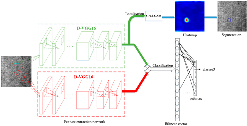
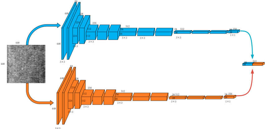
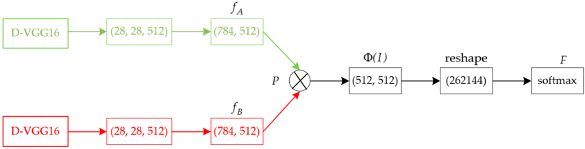
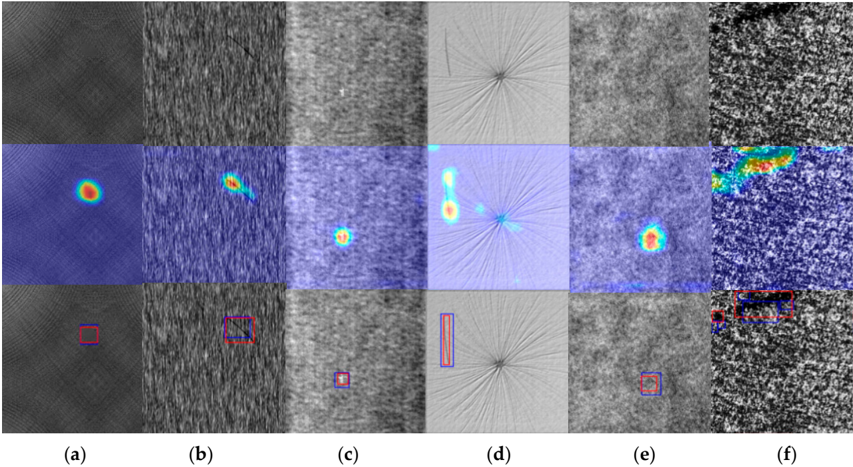
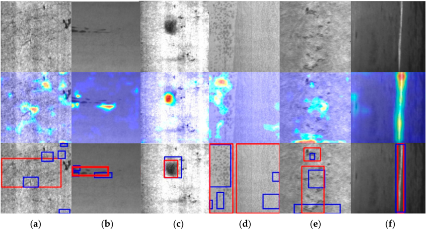
Aiming at the problems of complex texture, variable interference factors and large sample acquisition in surface defect detection, a generic method of automated surface defect detection based on a bilinear model was proposed. To realize the automatic classification and localization of surface defects, a new Double-Visual Geometry Group16 (D-VGG16) is firstly designed as feature functions of the bilinear model. The global and local features fully extracted from the bilinear model by D-VGG16 are output to the soft-max function to realize the automatic classification of surface defects. Then the heat map of the original image is obtained by applying Gradient-weighted Class Activation Mapping (Grad-CAM) to the output features of D-VGG16. Finally, the defects in the original input image can be located automatically after processing the heat map with a threshold segmentation method. The training process of the proposed method is characterized by a small sample, end-to-end, and is weakly-supervised. Furthermore, experiments are performed on two public and two industrial datasets, which have different defective features in texture, shape and color. The results show that the proposed method can simultaneously realize the classification and localization of defects with different defective features. The average precision of the proposed method is above 99% on the four datasets, and is higher than the known latest algorithms.
Overview
The claims and statistics of this paper haven’t been checked yet.
Free: it reads the open-access text and checks the first 5 claims that cite a source we can check. Create a free account to check every claim.
Integrity signals
Registry
Cites
Statistics
Figures

Verification
Claims the paper makes
The claims and statistics of this paper haven’t been checked yet.
Free: it reads the open-access text and checks the first 5 claims that cite a source we can check. Create a free account to check every claim.
Self-check
Percentages, sums and reported differences re-computed from the paper’s own numbers.
The self-check needs the paper’s full text.
Citations
Cites
Very Deep Convolutional Networks for Large-Scale Image Recognition
Simonyan, K., & Zisserman, A. (2014) · arXiv · doi:10.48550/arxiv.1409.1556 · Cited by 114,148
Adam: A Method for Stochastic Optimization
Kingma, D. P., & Ba, J. (2014) · arXiv · doi:10.48550/arxiv.1412.6980 · Cited by 98,946
Faster R-CNN: Towards Real-Time Object Detection with Region Proposal Networks
Ren, S., He, K., Girshick, R., & Sun, J. (2017) · IEEE Transactions on Pattern Analysis and Machine Intelligence · doi:10.1109/tpami.2016.2577031 · Cited by 73,472
Faster R-CNN: Towards Real-Time Object Detection with Region Proposal Networks
Ren, S., He, K., Girshick, R., & Sun, J. (2015) · arXiv · doi:10.48550/arxiv.1506.01497 · Cited by 70,812
ImageNet: A large-scale hierarchical image database
Deng, J., Dong, W., Socher, R., Li, L.-J., Li, K., & Fei-Fei, L. (2009) · 2009 IEEE Conference on Computer Vision and Pattern Recognition · doi:10.1109/cvpr.2009.5206848 · Cited by 65,333
A Threshold Selection Method from Gray-Level Histograms
Otsu, N. (1979) · IEEE Transactions on Systems, Man, and Cybernetics · doi:10.1109/tsmc.1979.4310076 · Cited by 43,398
(2016) · Cited by 31,590
Grad-CAM: Visual Explanations from Deep Networks via Gradient-Based Localization
Selvaraju, R. R., Cogswell, M., Das, A., Vedantam, R., Parikh, D., & Batra, D. (2017) · 2017 IEEE International Conference on Computer Vision (ICCV) · doi:10.1109/iccv.2017.74 · Cited by 24,513
SSD: Single Shot MultiBox Detector
Liu, W., Anguelov, D., Erhan, D., Szegedy, C., Reed, S., Fu, C.-Y., & Berg, A. C. (2016) · Lecture Notes in Computer Science · doi:10.1007/978-3-319-46448-0_2 · Cited by 22,128
Multiresolution gray-scale and rotation invariant texture classification with local binary patterns
Ojala, T., Pietikainen, M., & Maenpaa, T. (2002) · IEEE Transactions on Pattern Analysis and Machine Intelligence · doi:10.1109/tpami.2002.1017623 · Cited by 15,398
Learning Deep Features for Discriminative Localization
Zhou, B., Khosla, A., Lapedriza, A., Oliva, A., & Torralba, A. (2016) · 2016 IEEE Conference on Computer Vision and Pattern Recognition (CVPR) · doi:10.1109/cvpr.2016.319 · Cited by 11,428
Bilinear CNN Models for Fine-Grained Visual Recognition
Lin, T.-Y., RoyChowdhury, A., & Maji, S. (2015) · 2015 IEEE International Conference on Computer Vision (ICCV) · doi:10.1109/iccv.2015.170 · Cited by 2,135
Cha, Y., Choi, W., Suh, G., Mahmoudkhani, S., & Büyüköztürk, O. (2018) · Computer-Aided Civil and Infrastructure Engineering · doi:10.1111/mice.12334 · Cited by 1,558 · cited 6×
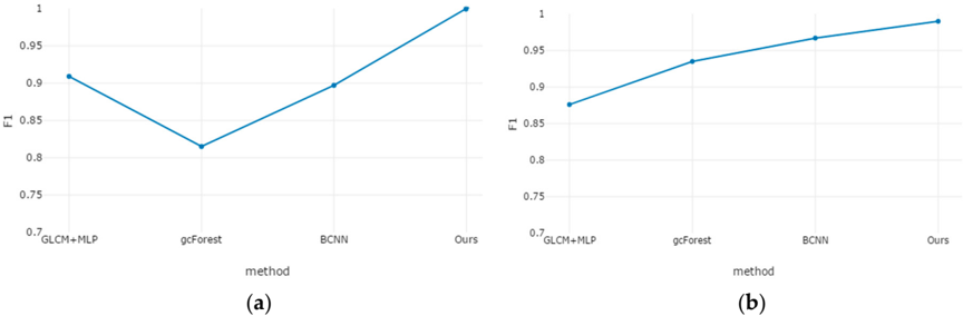
“Therefore, in each defect data set, not only GLCM + MLP [17], gcForest [32] and Bilinear Convolutional Neural Network (BCNN) are used to perform four kinds of generic surface defect detection algorithms, but also the open datasets will also be compared with the known latest experimental results on this dataset”
MethodResultInfluentialSong, K., & Yan, Y. (2013) · Applied Surface Science · doi:10.1016/j.apsusc.2013.09.002 · Cited by 1,026 · cited 1×
“The first open dataset is the DAGM_2007 surface defect dataset, which is manually generated and can be used for surface defect detection.”
MethodDeep Forest: Towards An Alternative to Deep Neural Networks
Zhou, Z.-H., & Feng, J. (2017) · Proceedings of the Twenty-Sixth International Joint Conference on Artificial Intelligence · doi:10.24963/ijcai.2017/497 · Cited by 935
A Generic Deep-Learning-Based Approach for Automated Surface Inspection
Ren, R., Hung, T., & Tan, K. C. (2018) · IEEE Transactions on Cybernetics · doi:10.1109/tcyb.2017.2668395 · Cited by 485
Automatic Metallic Surface Defect Detection and Recognition with Convolutional Neural Networks
Tao, X., Zhang, D., Ma, W., Liu, X., & Xu, D. (2018) · Applied Sciences · doi:10.3390/app8091575 · Cited by 471 · cited 1×
“The whole network is a typical bilinear model structure.”
BackgroundAutomatic Defect Detection on Hot-Rolled Flat Steel Products
Ghorai, S., Mukherjee, A., Gangadaran, M., & Dutta, P. K. (2013) · IEEE Transactions on Instrumentation and Measurement · doi:10.1109/tim.2012.2218677 · Cited by 317
Automatic watershed segmentation of randomly textured color images
Shafarenko, L., Petrou, M., & Kittler, J. (1997) · IEEE Transactions on Image Processing · doi:10.1109/83.641413 · Cited by 308
Attention-Guided Unified Network for Panoptic Segmentation
Li, Y., Chen, X., Zhu, Z., Xie, L., Huang, G., Du, D., & Wang, X. (2019) · 2019 IEEE/CVF Conference on Computer Vision and Pattern Recognition (CVPR) · doi:10.1109/cvpr.2019.00719 · Cited by 262
Automated defect inspection of LED chip using deep convolutional neural network
Lin, H., Li, B., Wang, X., Shu, Y., & Niu, S. (2019) · Journal of Intelligent Manufacturing · doi:10.1007/s10845-018-1415-x · Cited by 241
Surface defect classification of steels with a new semi-supervised learning method
Di, H., Ke, X., Peng, Z., & Dongdong, Z. (2019) · Optics and Lasers in Engineering · doi:10.1016/j.optlaseng.2019.01.011 · Cited by 241 · cited 1×
“The whole network is a typical bilinear model structure.”
BackgroundZhao, M. J., Lin, J., Miao, Y., & Xu, X. (2016) · Measurement · doi:10.1016/j.measurement.2016.05.068 · Cited by 152
A Surface Defect Detection Method Based on Positive Samples
Zhao, Z., Li, B., Dong, R., & Zhao, P. (2018) · Lecture Notes in Computer Science · doi:10.1007/978-3-319-97310-4_54 · Cited by 142
Multi-Object Tracking with Multiple Cues and Switcher-Aware Classification
Feng, W., Hu, Z., Wu, W., Yan, J., & Ouyang, W. (2019) · arXiv (Cornell University) · doi:10.48550/arxiv.1901.06129 · Cited by 82
Fully Convolutional Networks for Surface Defect Inspection in Industrial Environment
Yu, Z., Wu, X., & Gu, X. (2017) · Lecture Notes in Computer Science · doi:10.1007/978-3-319-68345-4_37 · Cited by 77 · cited 4×
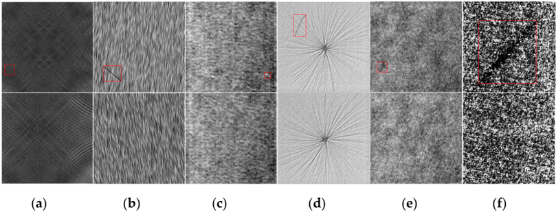
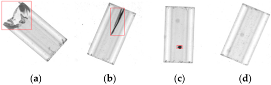
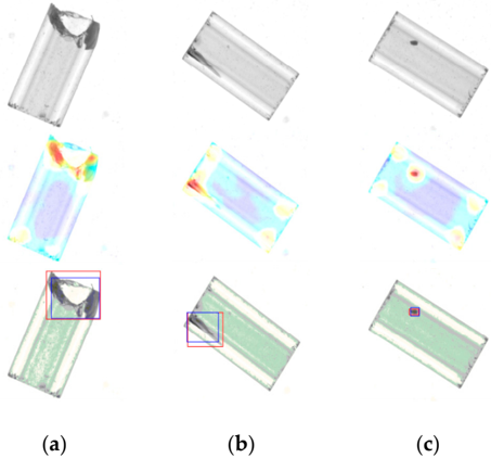
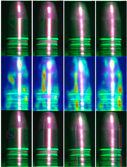
“…and Classification Results of the Diode Glass Bulb Surface Defect Dataset: For the diode glass bulb surface defect dataset, the ratio of the training set and testing set images Some experimental localization results of defect detection on this dataset by the proposed method are shown in Figure…”
MethodInfluentialAn evolutionary classifier for steel surface defects with small sample set
Xiao, M., Jiang, M., Li, G., Xie, L., & Yi, L. (2017) · EURASIP Journal on Image and Video Processing · doi:10.1186/s13640-017-0197-y · Cited by 55 · cited 2×
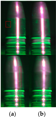
“Some experimental localization results of defect detection on this dataset by the proposed method are shown in ] 98 ] 99 Ours 99.44%”
BackgroundMethodInfluentialVerifying edges for visual inspection purposes
Wen, W., & Xia, A. (1999) · Pattern Recognition Letters · doi:10.1016/s0167-8655(98)00150-0 · Cited by 48
Artetxe, E., Olvera, D., de Lacalle, L. N. L., Campa, F. J., Olvera, D., & Lamíkiz, A. (2016) · The International Journal of Advanced Manufacturing Technology · doi:10.1007/s00170-016-9435-1 · Cited by 47
Inspection scheduling based on reliability updating of gas turbine welded structures
Coro, A., Abasolo, M., Aguirrebeitia, J., & de Lacalle, L. N. L. (2019) · Advances in Mechanical Engineering · doi:10.1177/1687814018819285 · Cited by 37
Steel Surface Defects Detection Based on Deep Learning
Lin, W.-Y., Lin, C., Chen, G.-S., & Hsu, C.-Y. (2018) · Advances in intelligent systems and computing · doi:10.1007/978-3-319-94484-5_15 · Cited by 23
Surface Defect Recognition for Metals Based on Feature Fusion of Shearlets and Wavelets
Zhou, P. (2015) · Journal of Mechanical Engineering · doi:10.3901/jme.2015.06.098 · Cited by 11
Research works printed but not linked: 5
- Santoyo, 2019, Reconocimiento de patrones y evaluación del daño generado en aceros de baja aleación a partir del procesamiento digital de imágenes e inteligencia artificial, DYNA Ing. Ind., 94, 357
- Lin, M., Chen, Q., and Yan, S. (2013, January 2–4). Network in network. Proceedings of the International Conference on Learning Representations (ICLR), Scottsdale, AZ, USA.
- Yosinski, J., Clune, J., Bengio, Y., and Lipson, H. How transferable are features in deep neural networks? In Proceedings of the Advances in Neural Information Processing Systems, Montreal, QC, Canada, 8–13 December 2014; pp.
- Ostu, 1975, A threshold selection method from gray-histogram, IEEE Trans. Syst. Man Cybern., 9, 62
- Song, 2014, Automatic recognition of surface defects on hot-rolled steel strip using scattering convolution network, J. Comput. Inf. Syst., 10, 3049
Cited by
Automated Visual Defect Detection for Flat Steel Surface: A Survey
Luo, Q., Fang, X., Liu, L., Yang, C., & Sun, Y. (2020) · IEEE Transactions on Instrumentation and Measurement · doi:10.1109/tim.2019.2963555 · Cited by 559
Deep CNN-based visual defect detection: Survey of current literature
Jha, S. B., & Babiceanu, R. F. (2023) · Computers in Industry · doi:10.1016/j.compind.2023.103911 · Cited by 224
Steel Surface Defect Recognition: A Survey
Wen, X., Shan, J., He, Y., & Song, K. (2022) · Coatings · doi:10.3390/coatings13010017 · Cited by 210
Research Progress of Automated Visual Surface Defect Detection for Industrial Metal Planar Materials
Fang, X., Luo, Q., Zhou, B., Li, C., & Tian, L. (2020) · Sensors · doi:10.3390/s20185136 · Cited by 160
A lightweight detector based on attention mechanism for aluminum strip surface defect detection
Ma, Z., Li, Y., Huang, M., Huang, Q., Cheng, J., & Tang, S. Y. (2021) · Computers in Industry · doi:10.1016/j.compind.2021.103585 · Cited by 131
Metadata
- Authors
- Zhou, F., Liu, G., Xu, F., & Deng, H.
- Affiliations
- Southwest University of Science and Technology (CN)
- Corresponding author
- Liu, Guihua
- Venue
- Applied Sciences
- Publisher
- MDPI AG
- Published
- 2019-08-03
- Volume
- 9
- Issue
- 15
- Pages
- 3159
- ISSN
- 2076-3417 (ISSN-L)
- OpenAlex
- W2965258271
- Semantic Scholar
- 08b361036d68c16a57a1b17e0d623ef10a02d4ee
- Cited by
- 47
- References
- 33
- Citations by year
- 2026: 2 · 2025: 4 · 2024: 7 · 2023: 7 · 2022: 8 · 2021: 10 · 2020: 8 · 2019: 1
- FWCI
- 4.98
- Type
- journal article
- Language
- en
- Open access
- gold
- dx.doi.org
- Licence
- Locations
- Applied Sciences (publishedVersion, cc-by)
- DOAJ (DOAJ: Directory of Open Access Journals) (submittedVersion)
- Funders
- National Natural Science Foundation of China (11602292, 61701421, 61601381)
- Topics
- Physical Sciences › Engineering › Industrial and Manufacturing Engineering › Industrial Vision Systems and Defect Detection
- Physical Sciences › Engineering › Mechanical Engineering › Non-Destructive Testing Techniques
- Physical Sciences › Engineering › Civil and Structural Engineering › Infrastructure Maintenance and Monitoring
- Keywords
- surface defect detection, bilinear model, Grad-CAM, heatmaps, defect localization, defect classification, weakly supervised learning, end-to-end learning, thresholding, industrial inspection
About these checks
Registry, retraction, Cites and statistics results are computed, not judged, with one exception: a printed reference that no index lists is read once by a model before it counts as a citation error. Claims are extracted by a model and kept only when their quote appears verbatim in the text; each cited source is then checked, with a model’s help, for whether it says what the claim relies on. Those verdicts can be wrong — read the claim’s quote and the cited source before relying on one.
Statistics and arithmetic are recomputed, not judged.
Confidence bands are shown only for fields calibrated on our annotated test set. None is calibrated yet, so no band is shown.
What counts as a claim ›How we measure confidence ›How we check this ›
Are you an author, or do you see a problem with this page? Request a review
Data sources
Bibliographic data: Semantic Scholar, OpenAlex, Crossref.
Contains information from the Semantic Scholar Academic Graph Datasets, made available under the ODC Attribution License (ODC-BY 1.0).
Semantic Scholar’s data is described in: Kinney, R., et al. (2023). The Semantic Scholar Open Data Platform. arXiv:2301.10140.
