

Epistemic Communities under Active Inference
Open accessThe DOI matches its Crossref record; 165 of the 165 references it cites were found in a registry or an index; 7 of the 18 sources its claims cite were checked for support.
Abstract
The spread of ideas is a fundamental concern of today’s news ecology. Understanding the dynamics of the spread of information and its co-option by interested parties is of critical importance. Research on this topic has shown that individuals tend to cluster in echo-chambers and are driven by confirmation bias. In this paper, we leverage the active inference framework to provide an in silico model of confirmation bias and its effect on echo-chamber formation. We build a model based on active inference, where agents tend to sample information in order to justify their own view of reality, which eventually leads to them to have a high degree of certainty about their own beliefs. We show that, once agents have reached a certain level of certainty about their beliefs, it becomes very difficult to get them to change their views. This system of self-confirming beliefs is upheld and reinforced by the evolving relationship between an agent’s beliefs and observations, which over time will continue to provide evidence for their ingrained ideas about the world. The epistemic communities that are consolidated by these shared beliefs, in turn, tend to produce perceptions of reality that reinforce those shared beliefs. We provide an active inference account of this community formation mechanism. We postulate that agents are driven by the epistemic value that they obtain from sampling or observing the behaviours of other agents. Inspired by digital social networks like Twitter, we build a generative model in which agents generate observable social claims or posts (e.g., ‘tweets’) while reading the socially observable claims of other agents that lend support to one of two mutually exclusive abstract topics. Agents can choose which other agent they pay attention to at each timestep, and crucially who they attend to and what they choose to read influences their beliefs about the world. Agents also assess their local network’s perspective, influencing which kinds of posts they expect to see other agents making. The model was built and simulated using the freely available Python package pymdp. The proposed active inference model can reproduce the formation of echo-chambers over social networks, and gives us insight into the cognitive processes that lead to this phenomenon.
Overview
CoChat Summary
## TL;DR
This paper presents a multi-agent active inference model of opinion dynamics in which agents infer both an abstract binary “Idea” and other agents’ beliefs from observable “Hashtags,” and use those inferences to choose whom to attend to and what to tweet. Simulations show that epistemic confirmation bias, network connectivity, inverse social volatility, and habit learning jointly shape whether groups polarize into echo-chambers or converge toward consensus.
## Key findings
- The model reproduces confirmation-bias-like dynamics: higher epistemic confirmation bias \(\gamma\) makes agents preferentially sample like-minded neighbours and can drive echo-chamber formation.
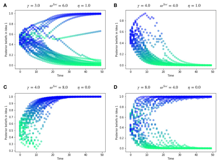
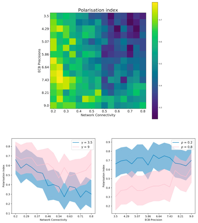
- In the network experiments, increasing connectivity \(p\) generally reduced polarisation, but high \(\gamma\) could counteract this: even at \(p=0.8\), many trials still ended in polarised dynamics.
- For the \(\gamma\)–\(\omega_{\mathrm{Soc}}\) sweep, the authors report 15 values of \(\gamma\) over \((3,9)\), 15 values of \(\omega_{\mathrm{Soc}}\) over \((0.05,1.0)\), \(N=15\) agents, and \(p=0.4\); low inverse social volatility led to more re-attendance to neighbours.
- In the habit-formation experiment, higher learning rate \(\eta\) increased polarisation; the average re-attendance rate was “seemingly maximised” when \(\eta \approx 0.3\), and the effect was strongest at high \(\gamma\) and \(\eta\).
## Methods
- Multi-agent simulations were built under a discrete active inference/POMDP framework, with agents inferring an abstract binary hidden state (“Idea 1” vs “Idea 2”), neighbours’ meta-beliefs, and their own actions from observed tweets/hashtags.
- The simulations used Erdős–Rényi networks and the freely available Python package `pymdp`; network size ranged from \(N=12\)–30 in general, and the main quantitative experiments used \(N=15\) agents with 100 independent realisations per condition and \(T=100\) timesteps.
- Main analyses were parameter sweeps over epistemic confirmation bias \(\gamma\), inverse social volatility \(\omega_{\mathrm{Soc}}\), habit-learning rate \(\eta\), and connectivity \(p\), with outcomes summarized using polarisation index \(\rho\) and re-attendance rate \(r\).
## Limitations
- The paper states that the parameter search “was not exhaustive,” and that large regions of parameter space remain unexplored.
- It states that network size was largely fixed/small for computational reasons: simulations mainly used \(N=30\) or \(N=15\), \(\omega_{\mathrm{Idea}}=9.0\) was fixed, and the authors say results are not guaranteed to generalise to larger networks.
- It also says the outcome measures were relatively simple: the polarisation metric is one-dimensional and does not distinguish different belief-network configurations. Evidence from the text also makes clear that the model omits any true environmental signal and only models two mutually exclusive Ideas; this is a modeling simplification the authors themselves acknowledge as needing future extension.
Model-written summary. Check it against the paper before relying on it.
Integrity signals
Registry
Cites
Statistics
Figures




Verification
Claims the paper makes
5 Valid · 2 Not valid · 5 Not checked · 112 Own results and interpretations
The cited sources support only part of this claim — read each source’s verdict below.
In the paper
“However, clearly defined clusters and group boundaries can sometimes act as buffers [132,133,134,135,136].”
§ Epistemic Communities under Active Inference > 5. Discussion
What the sources say
- Not checked — no full text of the sourcecites [132] Almogren, 2019, An efficient networking protocol for internet of things to handle multimedia big data, Multimed. Tools Appl. source
- Not checked — no full text of the sourcecites [133] 2005, Gated communities: Sprawl and social segregation in Southern California, Hous. Stud. source
- Not checked — no full text of the sourcecites [134] Aldrich, 1977, Boundary spanning roles and organization structure, Acad. Manag. Rev. source
- Partly supportedcites [135] Jaemthaworn, 2021, Topological clustering of regulatory genes confers pathogenic tolerance to cassava brown streak virus (CBSV) in cassava, Sci. Rep. sourceExperimental — accuracy not yet measured
The Results section on microscopic-scale clustered topology says that a highly connected gene-cluster structure buffered network disruption during simulated perturbation. It does not show that clearly defined group boundaries themselves act as buffers; the protective feature studied was connectivity within gene clusters. (LLM, conf=0.85)
- Not checked — no full text of the sourcecites [136] Richter, 2006, Boundary spanners’ identification, intergroup contact, and effective intergroup relations, Acad. Manag. J. source
boostedstates a possible cause- Asserted: passes — The authors put it forward as true.
- Checkable: passes — It can be checked against evidence.
- Load-bearing: passes — The paper’s conclusions depend on it.
- Based: passes — The paper gives a reason why it holds.
A result the paper reports from its own data — it cites no other source for it, so there is none to check. The quote shows it is in the paper.
In the paper
“With high enough γ or high enough ωSoc, the focal agent’s beliefs, faced with these two conflicting sources of information, converge to one Idea.”
§ Epistemic Communities under Active Inference > 4. Results > 4.1. Opinion Formation in a Single Agent
plainstates a cause- Asserted: passes — The authors put it forward as true.
- Checkable: passes — It can be checked against evidence.
- Load-bearing: passes — The paper’s conclusions depend on it.
- Based: passes — The paper gives a reason why it holds.
- Rests on 3 assumptions not shown here.
A result the paper reports from its own data — it cites no other source for it, so there is none to check. The quote shows it is in the paper.
In the paper
“In general, Figure 2 shows that beliefs in more meta-belief volatility (lower ωSoc) lead to higher posterior uncertainty about the sIdea hidden state, as is shown by the red lines in subplots (a) and (c).”
§ Epistemic Communities under Active Inference > 4. Results > 4.1. Opinion Formation in a Single Agent
plainstates a cause- Asserted: passes — The authors put it forward as true.
- Checkable: passes — It can be checked against evidence.
- Load-bearing: unclear — It is unclear whether the paper’s conclusions depend on it.
- Based: passes — The paper gives a reason why it holds.
- Rests on 3 assumptions not shown here.
A result the paper reports from its own data — it cites no other source for it, so there is none to check. The quote shows it is in the paper.
In the paper
“The proposed active inference model can reproduce the formation of echo-chambers over social networks, and gives us insight into the cognitive processes that lead to this phenomenon.”
§ Epistemic Communities under Active Inference > Abstract
plainstates a cause- Asserted: passes — The authors put it forward as true.
- Checkable: passes — It can be checked against evidence.
- Load-bearing: passes — The paper’s conclusions depend on it.
- Based: passes — The paper gives a reason why it holds.
A result the paper states — it cites no source for it, so there is none to check. The quote shows it is in the paper.
In the paper
“We show that, once agents have reached a certain level of certainty about their beliefs, it becomes very difficult to get them to change their views.”
§ Epistemic Communities under Active Inference > Abstract
plainstates a cause- Asserted: passes — The authors put it forward as true.
- Checkable: passes — It can be checked against evidence.
- Load-bearing: passes — The paper’s conclusions depend on it.
- Based: passes — The paper gives a reason why it holds.
82 more claims
Create a free account to see all 124 claims and to verify the 1 reference still open.
- Probably not a substantial claim. 21
- It may state two separate claims as one. 19
Citations
Cites
The need to belong: Desire for interpersonal attachments as a fundamental human motivation.
Baumeister, R. F., & Leary, M. R. (1995) · Psychological Bulletin · doi:10.1037//0033-2909.117.3.497 · Cited by 23,245 · cited 1×
“The spread of ideas and behaviors from one agent to another serves 77 both local and larger-scale coordination [28,29].”
BackgroundThe Proceedings of the National Academy of Sciences
Richards, J. W. (1915) · Science · doi:10.1126/science.42.1074.161 · Cited by 13,983
Markov decision processes: Discrete stochastic dynamic programming
Hazeghi, K., & Puterman, M. L. (1995) · Journal of the American Statistical Association · doi:10.2307/2291177 · Cited by 8,037
International Journal of Environmental Research and Public Health
(2013) · International Journal of Environmental Research and Public Health · doi:10.3390/ijerph · Cited by 7,753
Social Influence: Compliance and Conformity
Cialdini, R. B., & Goldstein, N. J. (2004) · Annual Review of Psychology · doi:10.1146/annurev.psych.55.090902.142015 · Cited by 6,077 · cited 1×
“This is partly due to the fact that members of an in-group can be most precisely predicted: their behaviours are normed, and expected by the members of the group, in ways that generally benefit its members [18,19].”
BackgroundTaking the Human Out of the Loop: A Review of Bayesian Optimization
Shahriari, B., Swersky, K., Wang, Z., Adams, R. P., & de Freitas, N. (2016) · Proceedings of the IEEE · doi:10.1109/jproc.2015.2494218 · Cited by 6,049
Markov Decision Processes: Discrete Stochastic Dynamic Programming
Puterman, M. L. (1994) · Wiley Series in Probability and Statistics · doi:10.1002/9780470316887 · Cited by 6,024
Journal of the American Statistical Association
Koehler, A. B. (1995) · International Journal of Forecasting · doi:10.1016/0169-2070(95)90067-5 · Cited by 5,337
MacKay, D. J. C. (1992) · Neural Computation · doi:10.1162/neco.1992.4.3.415 · Cited by 4,388 · cited 1×
“The remaining (negative) surprise can be 371 itself used as a score for model averaging and model selection [118,119].”
Motivated Skepticism in the Evaluation of Political Beliefs
Taber, C. S., & Lodge, M. (2006) · American Journal of Political Science · doi:10.1111/j.1540-5907.2006.00214.x · Cited by 4,344
Research works printed but not linked: 5
- Heerwagen, 1995, Humans, habitats, Biophilia Hypothesis, 138, 138
- Oswald, M.E., and Grosjean, S. (2004). Confirmation bias. Cognitive Illusions: A Handbook on Fallacies and Biases in Thinking, Judgement and Memory, Psychology Press.
- Ladegard, 2006, Accessing Social Capital through Conformity: Investigating Network Cultures, Adv. Organ. Stud., 20, 153
- Gumperz, 2009, The speech community, Linguist. Anthropol. A Read., 1, 66
- Sutton, R.S., and Barto, A.G. (2018). Reinforcement Learning: An Introduction, MIT Press.
Cited by
Collective behavior from surprise minimization
Heins, C., Millidge, B., Da Costa, L., Mann, R. P., Friston, K. J., & Couzin, I. D. (2024) · Proceedings of the National Academy of Sciences · doi:10.1073/pnas.2320239121 · Cited by 55
Self-citationCognition as Morphological/Morphogenetic Embodied Computation In Vivo
Dodig-Crnković, G. (2022) · Entropy · doi:10.3390/e24111576 · Cited by 48
“These lines of inquiry range from the nature of dyadic interactions to the spread of ideas over communities, [110,111].”
BackgroundDesigning ecosystems of intelligence from first principles
Friston, K. J., Ramstead, M. J. D., Kiefer, A. B., Tschantz, A., Buckley, C. L., Albarracin, M., Pitliya, R. J., Heins, C., Klein, B., Millidge, B., et al. (2024) · Collective Intelligence · doi:10.1177/26339137231222481 · Cited by 94
“Heuristically, maximizing model evidence means making the world as predictable as possible (Albarracin et al., 2022; Kastel and Hesp, 2021).”
BackgroundSelf-citationNarrative as active inferencePreprint
Bouizegarene, N., Ramstead, M. J. D., Constant, A., Friston, K. J., & Kirmayer, L. J. (2020) · doi:10.31234/osf.io/47ub6 · Cited by 34
Self-citationAesthetics and predictive processing: grounds and prospects of a fruitful encounter
Frascaroli, J., Leder, H., Brattico, E., & de Cruys, S. V. (2023) · Philosophical Transactions of the Royal Society B Biological Sciences · doi:10.1098/rstb.2022.0410 · Cited by 54
Federated inference and belief sharing
Friston, K. J., Parr, T., Heins, C., Constant, A., Friedman, D., Isomura, T., Fields, C., Verbelen, T., Ramstead, M., Clippinger, J., et al. (2024) · Neuroscience & Biobehavioral Reviews · doi:10.1016/j.neubiorev.2023.105500 · Cited by 30
Self-citationPezzulo, G., D’Amato, L., Mannella, F., Priorelli, M., de Maele, T. V., Stoianov, I. P., & Friston, K. J. (2024) · Annals of the New York Academy of Sciences · doi:10.1111/nyas.15118 · Cited by 32
Collective Intelligence in Human-AI Teams: A Bayesian Theory of Mind Approach
Westby, S., & Riedl, C. (2023) · Proceedings of the AAAI Conference on Artificial Intelligence · doi:10.1609/aaai.v37i5.25755 · Cited by 59
Resilience and active inference
Miller, M. M., Albarracin, M., Pitliya, R. J., Kiefer, A. B., Mago, J., Gorman, C., Friston, K. J., & Ramstead, M. J. D. (2022) · Frontiers in Psychology · doi:10.3389/fpsyg.2022.1059117 · Cited by 27
Self-citationFeeling our place in the world: an active inference account of self-esteem
Albarracin, M., Bouchard-Joly, G., Sheikhbahaee, Z., Miller, M. D., Pitliya, R. J., & Poirier, P. (2024) · Neuroscience of Consciousness · doi:10.1093/nc/niae007 · Cited by 37
Self-citationThe nature of beliefs and believing
Albarracin, M., & Pitliya, R. J. (2022) · Frontiers in Psychology · doi:10.3389/fpsyg.2022.981925 · Cited by 20
“misinformation on social media, spreading extremely fast in echo-chambers, and leading to radicalization (Albarracin et al., 2022).”
BackgroundSelf-citationKirmayer, L. J. (2024) · Transcultural Psychiatry · doi:10.1177/13634615241296301 · Cited by 21
As One and Many: Relating Individual and Emergent Group-Level Generative Models in Active Inference
Waade, P. T., Olesen, C., Laursen, J. E., Nehrer, S. W., Heins, C., Friston, K. J., & Mathys, C. D. (2025) · Entropy · doi:10.3390/e27020143 · Cited by 16
“…the preference for being aligned with interlocutors—is observed in in vivo neurons [42–44] and can be a mechanism for implementing cumulative culture [45,46], which can also lead to separate echo-chamber-like epistemic communities that maintain highly precise and difficult-to-change beliefs [47].”
Self-citationSpin Glass Systems as Collective Active Inference
Heins, C., Klein, B., Demekas, D., Aguilera, M., & Buckley, C. L. (2023) · Communications in computer and information science · doi:10.1007/978-3-031-28719-0_6 · Cited by 19
Self-citationFrom the Evaluator’s Perspective: A Functional Approach to Social Judgments
Bitektine, A. B., Gillespie, N. A., & Lange, D. A. (2025) · Academy of Management Review · doi:10.5465/amr.2020.0405 · Cited by 14
Frauhammer, L. T., & Neubaum, G. (2023) · Frontiers in Psychology · doi:10.3389/fpsyg.2023.1146674 · Cited by 10
“org confirmation bias or the formation of echo chambers (Albarracin et al., 2022).”
BackgroundSustainability under Active Inference
Albarracin, M., Ramstead, M. J. D., Pitliya, R. J., Hipólito, I., Costa, L. D., Raffa, M., Constant, A., & Manski, S. G. (2024) · Systems · doi:10.3390/systems12050163 · Cited by 14
Self-citationResilience phenotypes derived from an active inference account of allostasis
Harrison, L., Gracias, A. J., Friston, K. J., & Buckwalter, J. G. (2025) · Frontiers in Behavioral Neuroscience · doi:10.3389/fnbeh.2025.1524722 · Cited by 12
Active Inference With Empathy Mechanism for Socially Behaved Artificial Agents in Diverse Situations
Matsumura, T., Esaki, K., Shao, Y., Yoshimura, C., & Mizuno, H. (2023) · Artificial Life · doi:10.1162/artl_a_00416 · Cited by 13
“Although active inference is basically defined for single-agent cases, some works have recently extended it to multiagent cases (Albarracin et al., 2022; Friedman et al., 2021; Kaufmann et al., 2021; Wirkuttis & Tani, 2021).”
BackgroundDeslatte, A., & Chung, J. (2025) · State and Local Government Review · doi:10.1177/0160323x241283407 · Cited by 8
“Extended to groups, exploratory evidence-gathering can provide epistemic gains which help resolve these discrepancies by facilitating experimentation and learning (Albarracin et al. 2022).”
The Inherent Normativity of Concepts
So, W. Y., Friston, K. J., & Neacsu, V. (2024) · Minds and Machines · doi:10.1007/s11023-024-09697-7 · Cited by 5
“In other words, the concepts an agent acquires through exchange with her world is quintessentially intersubjective, should that world be constituted by agents gathering evidence for their models of the shared world (Albarracin et al., 2022; Kastel & Hesp, 2021; Vasil et al., 2020).”
Krahé, C., Koukoutsakis, A., & Fotopoulou, A. (2024) · Cognition · doi:10.1016/j.cognition.2024.105756 · Cited by 4
“Epistemic trust refers to an individual's willingness to consider new information as trust-worthy, reliable, and salient (having high epistemic value; Albarracin, Demekas, Ramstead, & Heins, 2022).”
BackgroundGUÉNIN--CARLUT, A. (2022) · OSF Preprints (OSF Preprints) · doi:10.31219/osf.io/x7yr4 · Cited by 5
Distributed Science - The Scientific Process as Multi-Scale Active InferencePreprint
Balzan, F., Campbell, J. O., Friston, K. J., Ramstead, M. J. D., Friedman, D., & Constant, A. (2023) · OSF Preprints (OSF Preprints) · doi:10.31219/osf.io/dnw5k · Cited by 9
Self-citationNehrer, S. W., Laursen, J. E., Heins, C., Friston, K. J., Mathys, C. D., & Waade, P. T. (2025) · Entropy · doi:10.3390/e27010062 · Cited by 8
Self-citationSocial Media Platforms: Trading with Prediction Error Minimization for Your AttentionPreprint
Ciria, A., Albarracin, M., Miller, M., & Lara, B. (2022) · Preprints.org · doi:10.20944/preprints202209.0259.v1 · Cited by 5
Self-citationSeeing no evil? Social vulnerabilities, collective inference, and organizational divergence
Deslatte, A., Stokan, E., & Chung, J. (2025) · Journal of Public Administration Research and Theory · doi:10.1093/jopart/muaf034 · Cited by 3
Myth of objectivity and the origin of symbols
Rahman, S. (2023) · Frontiers in Sociology · doi:10.3389/fsoc.2023.1269621 · Cited by 5
“In short, in building our encultured world or generative models, we will try to provide an accurate account of the sensed world that is minimally complex in accord with Occam’s principle and try to share that worldview with everyone we choose to engage with (Albarracin et al., 2022).”
BackgroundAlbarracin, M., de Jager, S., & Hyland, D. (2025) · Entropy · doi:10.3390/e27050522 · Cited by 4
“…context of complex communication and social coordination, problems arise when dominant narratives prioritize, e.g., mere power acquisition in favor of self-preservation, which has been examined as leading to misinformation, echo chambers, and policy jus-tifications based on assumed conditions [45].”
Self-citationMöller, M., & Polani, D. (2023) · Interface Focus · doi:10.1098/rsfs.2023.0006 · Cited by 4
Collective behavior from surprise minimization
Heins, C., Millidge, B., Costa, L. D., et al. (2023) · White Rose Research Online (University of Leeds, The University of Sheffield, University of York) · doi:10.48550/arxiv.2307.14804 · Cited by 2
Self-citationBelief Sharing: A Blessing or a Curse
Çatal, O., de Maele, T. V., Pitliya, R. J., Albarracin, M., Pattisapu, C., & Verbelen, T. (2024) · Communications in computer and information science · doi:10.1007/978-3-031-77138-5_8 · Cited by 7
Self-citationThe Effectiveness of Learning Media in Waste Management
Tarigan, L. B., Rogaleli, Y. C. L., & Dukabain, O. M. (2024) · JURNAL INFO KESEHATAN · doi:10.31965/infokes.vol22.iss3.1480 · Cited by 1
“…in managing waste because by knowing the characteristics of food they are able to identify what information they are willing to understand (Albarracin et al. 2022) and can determine effective methods (Tarigan, Rogaleli, and Waangsir 2020), so as to increase participation (Br Tarigan and…”
Albarracin, M., & Pitliya, R. J. (2022) · Physics of Life Reviews · doi:10.1016/j.plrev.2022.07.003 · Cited by 1
Self-citationRamstead, M. J. D. (2024) · doi:10.21428/e2759450.e4bf505d · Cited by 1
Self-citationResilience and Active InferencePreprint
Miller, M. M., Albarracin, M., Pitliya, R. J., et al. (2022) · doi:10.31234/osf.io/vehq2
Self-citationActive Inference and Psychology of Expectations: A Study of Formalizing ViolEx
Raghuveer, D., & Endres, D. (2023) · Communications in computer and information science · doi:10.1007/978-3-031-28719-0_17
Active Blockference: cadCAD with Active Inference for Cognitive Systems Modeling
Smékal, J., Choudhury, A., Singh, A. K., Damaty, S. E., & Friedman, D. (2023) · Communications in computer and information science · doi:10.1007/978-3-031-28719-0_10
Friston, K. J. (2023) · Behavioral and Brain Sciences · doi:10.1017/s0140525x2200276x
Friston, K. J. (2023) · Physics of Life Reviews · doi:10.1016/j.plrev.2023.06.001
SKYNET 2023 Conception of the Artificial Super Intelligence Project. A System Approach. ver. 3Preprint
Novikov, A. (2023) · OSF Preprints (OSF Preprints) · doi:10.31219/osf.io/kqt9p
Cultural bodybuilding: The embodied influence of culture on perception and action
Albarracin, M. (2025) · The Psychology of learning and motivation/The psychology of learning and motivation · doi:10.1016/bs.plm.2025.02.002 · Cited by 1
Self-citationWidler, V., Kamińska, B., Martins, A. C. R., & Puga‐Gonzalez, I. (2026) · Computational social sciences · doi:10.1007/978-3-032-01373-6_10 · Cited by 3
The Game of Self: Identity and Experience as Active Inference
Hirsh, J. B. (2026) · Personality and Social Psychology Review · doi:10.1177/10888683261422344
Rahman, S., & Pashea, A. (2026) · Frontiers in Sociology · doi:10.3389/fsoc.2026.1646503
Miyano, S., & SHIONO, T. (2026) · Entropy · doi:10.3390/e28050491
“Work that is closely related to the current treatment includes the explicit modelling of belief sharing in epistemic communities [52,53].”
Predictive brains in hyperreal worlds: how XR exploits the indifference to being
Wood, G. M. D. O., & Kober, S. E. (2026) · AI & Society · doi:10.1007/s00146-026-03197-1
Wiechman, A., Deslatte, A., Koebele, E. A., García, M., & Anderies, J. M. (2026) · Journal of Public Administration Research and Theory · doi:10.1093/jopart/muag014 · Cited by 2
Safavi‐Abbasi, S., Tasker, R., Reyes, P. M., Doyle, B., Dibaj, P., & Venezia, E. (2026) · Frontiers in Public Health · doi:10.3389/fpubh.2026.1914023
de Jager, S., & Albarracin, M. (2026) · Topoi · doi:10.1007/s11245-026-10458-7 · Cited by 3
Self-citationBelief Functions Meet Quantum Logic: A Mathematical Framework for Coherence-Based Decision Theories
Fioretti, G. (2026) · Complexities · doi:10.3390/complexities2030022
Metadata
- Authors
- Albarracin, M., Demekas, D., Ramstead, M. J. D., & Heins, C.
- Affiliations
- Université du Québec à Montréal (CA)
- Imperial College London (GB)
- Wellcome Centre for Human Neuroimaging (GB)
- University of Konstanz (DE)
- Corresponding author
- Albarracin, Mahault
- Heins, Conor
- Venue
- Entropy
- Publisher
- MDPI AG
- Published
- 2022-03-29
- Volume
- 24
- Issue
- 4
- Pages
- 476
- ISSN
- 1099-4300 (ISSN-L)
- PMC
- PMC9027706
- OpenAlex
- W4220746083
- Cited by
- 60
- References
- 157
- Citations by year
- 2026: 15 · 2025: 10 · 2024: 14 · 2023: 15 · 2022: 6
- FWCI
- 5.00
- Type
- journal article
- Language
- en
- Open access
- gold
- doi.org
- Licence
- Locations
- Entropy (publishedVersion, cc-by)
- Preprints.org (submittedVersion, cc-by)
- PubMed Central (publishedVersion, cc-by)
- PubMed (publishedVersion)
- KOPS (University of Konstanz) (submittedVersion, cc-by)
- DOAJ (DOAJ: Directory of Open Access Journals) (submittedVersion, cc-by-sa)
- Funders
- U.S. Office of Naval Research (N00014-19-1-2556)
- Topics
- Life Sciences › Neuroscience › Cognitive Neuroscience › Embodied and Extended Cognition
- Social Sciences › Sociology and Political Science › Misinformation and Its Impacts
- Physical Sciences › Physics and Astronomy › Statistical and Nonlinear Physics › Opinion Dynamics and Social Influence
- Keywords
- active inference, confirmation bias, echo chambers, epistemic communities, belief updating, information dissemination, social networks, in silico models, belief certainty, generative models
About these checks
Registry, retraction, Cites and statistics results are computed, not judged, with one exception: a printed reference that no index lists is read once by a model before it counts as a citation error. Claims are extracted by a model and kept only when their quote appears verbatim in the text; each cited source is then checked, with a model’s help, for whether it says what the claim relies on. Those verdicts can be wrong — read the claim’s quote and the cited source before relying on one.
The claim verdicts this report counts are experimental: their accuracy is not yet measured.
A language model drew the claims from the paper on 2026-10-06, under version 3 of the claim definition (model deepseek-v4.1-flash, prompt extract-v3).
A second model labelled each claim on 2026-10-06 (model jev-1.13-20260917, definition revision gold-guideline-v0.2).
Cited sources are checked with a language model’s help (gpt-6-sol).
Statistics and arithmetic are recomputed, not judged.
Confidence bands are shown only for fields calibrated on our annotated test set. None is calibrated yet, so no band is shown.
What counts as a claim ›How we measure confidence ›How we check this ›
Are you an author, or do you see a problem with this page? Request a review
Data sources
Bibliographic data: Semantic Scholar, OpenAlex, Crossref.
Contains information from the Semantic Scholar Academic Graph Datasets, made available under the ODC Attribution License (ODC-BY 1.0).
Semantic Scholar’s data is described in: Kinney, R., et al. (2023). The Semantic Scholar Open Data Platform. arXiv:2301.10140.
