

The suitability of differentiable, physics-informed machine learning hydrologic models for ungauged regions and climate change impact assessment
Open accessPublished version of a preprint
The DOI matches its Crossref record; 67 of the 67 references it cites were found in a registry or an index; 4 of the 27 sources its claims cite were checked for support.
Abstract
As a genre of physics-informed machine learning, differentiable process-based hydrologic models (abbreviated as δ or delta models) with regionalized deep-network-based parameterization pipelines were recently shown to provide daily streamflow prediction performance closely approaching that of state-of-the-art long short-term memory (LSTM) deep networks. Meanwhile, δ models provide a full suite of diagnostic physical variables and guaranteed mass conservation. Here, we ran experiments to test (1) their ability to extrapolate to regions far from streamflow gauges and (2) their ability to make credible predictions of long-term (decadal-scale) change trends. We evaluated the models based on daily hydrograph metrics (Nash–Sutcliffe model efficiency coefficient, etc.) and predicted decadal streamflow trends. For prediction in ungauged basins (PUB; randomly sampled ungauged basins representing spatial interpolation), δ models either approached or surpassed the performance of LSTM in daily hydrograph metrics, depending on the meteorological forcing data used. They presented a comparable trend performance to LSTM for annual mean flow and high flow but worse trends for low flow. For prediction in ungauged regions (PUR; regional holdout test representing spatial extrapolation in a highly data-sparse scenario), δ models surpassed LSTM in daily hydrograph metrics, and their advantages in mean and high flow trends became prominent. In addition, an untrained variable, evapotranspiration, retained good seasonality even for extrapolated cases. The δ models' deep-network-based parameterization pipeline produced parameter fields that maintain remarkably stable spatial patterns even in highly data-scarce scenarios, which explains their robustness. Combined with their interpretability and ability to assimilate multi-source observations, the δ models are strong candidates for regional and global-scale hydrologic simulations and climate change impact assessment.
Overview
CoChat Summary
TL;DR
The paper evaluates differentiable, physics-informed hydrologic models (δ models) against LSTM and a traditional regionalized model for spatial interpolation/extrapolation and long-term trend prediction on the CAMELS dataset. It finds that δ models generalize especially well in ungauged regions, with the two-parameter dynamic version δ(β_t, γ_t) performing best overall and retaining good evapotranspiration seasonality even under extrapolation.
Key findings
- On the randomized PUB test (531 basins), under Maurer forcings δ(β_t, γ_t) had median NSE 0.64 and LSTM had 0.65; for KGE, δ(β_t) and δ(β_t, γ_t) were 0.66 and 0.65, “essentially the same as LSTM,” but with a smaller spread.
- Under Daymet forcings in PUB, δ(β_t) and δ(β_t, γ_t) reached median NSE/KGE of 0.68/0.68 and 0.69/0.67, exceeding LSTM’s 0.66/0.66.
- In the regional holdout PUR test, δ models outperformed LSTM in most daily metrics; with Maurer forcings, median NSE/KGE were 0.55/0.52 for LSTM, 0.56/0.59 for δ, and 0.59/0.61 for δ(β_t, γ_t); with Daymet, they were 0.55/0.51, 0.60/0.61, and 0.62/0.63, respectively.
- For decadal trends in PUR, LSTM dropped sharply while δ models remained stable: LSTM annual-mean-flow R² fell from 0.87 (PUB) to 0.64 (PUR), and high-flow Q98 R² from 0.76 to 0.27, whereas δ(β_t, γ_t) stayed around 0.88 for annual mean discharge and about 0.77 for Q98 trends.
- For evapotranspiration, extrapolation had a moderate impact on seasonality and a muted impact on annual mean ET; under PUB/PUR the median correlation between simulated ET and MODIS ET stayed around 0.84 and RMSE around 6.4 mm per 8 d, with δ(γ_t, β_t) showing the best ET seasonality.
Methods
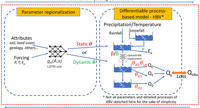
- The study used differentiable hydrologic models with an HBV backbone and neural-network parameterization; some versions included dynamic parameterization (DP) where β and γ became time-dependent (β_t, γ_t).
- Experiments were run on CAMELS basins across the contiguous United States: 671 basins for training and a 531-basin subset for reported test performance; PUB used 10 random folds, and PUR divided CONUS into seven regions with seven holdouts.
- Performance was evaluated using daily hydrograph metrics (NSE, KGE, FLV, FHV) and decadal streamflow trends (Sen’s slope for Q10, Q50, Q98, and mean annual flow); ET was independently checked against MODIS 8-day integrated ET.
Limitations
- The paper states that the comparison to an existing process-based model with parameter regionalization was only possible on the temporal test, because systematic PUB/PUR results for that model were not available.
- The authors note that the PUB setup was computationally economical and therefore less demanding than prior work: only 10 years of training were used, no ensemble was used, and a lower k-fold was used; they say stronger setups could be studied in future.
- Evident from the text: the study trains and evaluates on CONUS/CAMELS, so the conclusions about global applicability and data-poor continents are suggested rather than directly tested here.
Model-written summary. Check it against the paper before relying on it.
Integrity signals
Registry
Cites
Statistics
Figures



Verification
Claims the paper makes
3 Valid · 2 Not valid · 17 Not checked · 110 Own results and interpretations
The cited sources support only part of this claim — read each source’s verdict below.
In the paper
“Both the LSTM and δ models showed better performance when driven by Daymet forcings”
§ The suitability of differentiable, physics-informed machine learning hydrologic models for ungauged regions and climate change impact assessment > 3.1 The randomized PUB test
What the sources say
- Not matchedcites Feng et al., 2022a
More than one paper fits this citation.
- Partly supportedcites Kratzert et al., 2021 matched to “A note on leveraging synergy in multiple meteorological data sets with deep learning for rainfall–runoff modeling” (2021) sourceExperimental — accuracy not yet measured
The results discussion (around line 190) identifies DayMet as the best-performing single-forcing LSTM, supporting the LSTM part of the claim. The experimental design (section 2.3) describes LSTM models, but our copy does not report results for δ models, so their claimed improvement with DayMet is unsupported. (LLM, conf=0.88)
plainstates an association- Asserted: passes — The authors put it forward as true.
- Checkable: passes — It can be checked against evidence.
- Load-bearing: unclear — It is unclear whether the paper’s conclusions depend on it.
- Based: passes — The paper gives a reason why it holds.
- Not matched
The cited sources support only part of this claim — read each source’s verdict below.
In the paper
“This ET product served as a completely independent, uncalibrated validation for the evapotranspiration simulated by the differentiable HBV models.”
§ The suitability of differentiable, physics-informed machine learning hydrologic models for ungauged regions and climate change impact assessment > 2.3 Data
What the sources say
- Not matchedcites Mu et al., 2011
This doesn’t read as a citation we can look up.
- Partly supportedcites Running et al., 2017 matched to “MOD16A2 MODIS/Terra Net Evapotranspiration 8-Day L4 Global 500m SIN Grid V006” (2017) sourceExperimental — accuracy not yet measured
The Description identifies MOD16A2 as an evapotranspiration data product, supporting the identification of the ET product. It does not say that the product was used to validate differentiable HBV models or establish that such validation was completely independent and uncalibrated. (LLM, conf=0.84)
plain- Asserted: passes — The authors put it forward as true.
- Checkable: passes — It can be checked against evidence.
- Load-bearing: passes — The paper’s conclusions depend on it.
- Based: passes — The paper gives a reason why it holds.
- Not matched
A result the paper reports from its own data — it cites no other source for it, so there is none to check. The quote shows it is in the paper.
In the paper
“The median NSE (KGE) values for LSTM, δ, and δ(β t , γ t ) models were 0.55 (0.51), 0.60 (0.61) and 0.62 (0.63), respectively.”
§ The suitability of differentiable, physics-informed machine learning hydrologic models for ungauged regions and climate change impact assessment > 3.2 The region-based PUR test
plain- Asserted: passes — The authors put it forward as true.
- Checkable: passes — It can be checked against evidence.
- Load-bearing: passes — The paper’s conclusions depend on it.
- Based: passes — The paper gives a reason why it holds.
A result the paper reports from its own data — it cites no other source for it, so there is none to check. The quote shows it is in the paper.
In the paper
“The performance gap between LSTM and δ models was larger under Daymet forcings.”
§ The suitability of differentiable, physics-informed machine learning hydrologic models for ungauged regions and climate change impact assessment > 3.2 The region-based PUR test
plainstates an association- Asserted: passes — The authors put it forward as true.
- Checkable: passes — It can be checked against evidence.
- Load-bearing: unclear — It is unclear whether the paper’s conclusions depend on it.
- Based: passes — The paper gives a reason why it holds.
A result the paper reports from its own data — it cites no other source for it, so there is none to check. The quote shows it is in the paper.
In the paper
“The same pattern is obvious for the high flow (Q 98 ).”
§ The suitability of differentiable, physics-informed machine learning hydrologic models for ungauged regions and climate change impact assessment > 3.2 The region-based PUR test
plain- Asserted: passes — The authors put it forward as true.
- Checkable: passes — It can be checked against evidence.
- Load-bearing: unclear — It is unclear whether the paper’s conclusions depend on it.
- Based: passes — The paper gives a reason why it holds.
48 more claims
Create a free account to see all 132 claims and to verify the 2 references still open.
- It may state two separate claims as one. 55
- Probably not a substantial claim. 33
- The quote only partly states this claim. 6
Citations
Cites
River flow forecasting through conceptual models part I — A discussion of principles
Nash, J. E., & Sutcliffe, J. V. (1970) · Journal of Hydrology · doi:10.1016/0022-1694(70)90255-6 · Cited by 23,674
Estimates of the Regression Coefficient Based on Kendall's Tau
Sen, P. K. (1968) · Journal of the American Statistical Association · doi:10.1080/01621459.1968.10480934 · Cited by 14,517
Gupta, H. V., Kling, H., Yilmaz, K. K., & Martinez, G. F. (2009) · Journal of Hydrology · doi:10.1016/j.jhydrol.2009.08.003 · Cited by 6,758
Improvements to a MODIS global terrestrial evapotranspiration algorithm
Mu, Q., Zhao, M., & Running, S. W. (2011) · Remote Sensing of Environment · doi:10.1016/j.rse.2011.02.019 · Cited by 2,816
A manifesto for the equifinality thesis
Beven, K. (2006) · Journal of Hydrology · doi:10.1016/j.jhydrol.2005.07.007 · Cited by 2,581
Reassessing the projections of the World Water Development Report
Boretti, A., & Rosa, L. (2019) · npj Clean Water · doi:10.1038/s41545-019-0039-9 · Cited by 2,554
Estimates of the Regression Coefficient Based on Kendall's Tau
Sen, P. K. (1968) · Journal of the American Statistical Association · doi:10.2307/2285891 · Cited by 1,695
Maurer, E. P., Wood, A. W., Adam, J. C., Lettenmaier, D. P., & Nijssen, B. (2002) · Journal of Climate · doi:10.1175/1520-0442(2002)015<3237:althbd>2.0.co;2 · Cited by 1,441
A decade of Predictions in Ungauged Basins (PUB)—a review
Hrachowitz, M., Savenije, H. H. G., Blöschl, G., McDonnell, J. J., Sivapalan, M., Pomeroy, J. W., Arheimer, B., Blume, T., Clark, M. P., Ehret, U., et al. (2013) · Hydrological Sciences Journal · doi:10.1080/02626667.2013.803183 · Cited by 1,295
Kratzert, F., Klotz, D., Shalev, G., Klambauer, G., Hochreiter, S., & Nearing, G. (2019) · Hydrology and Earth System Sciences · doi:10.5194/hess-23-5089-2019 · Cited by 1,223
Research works printed but not linked: 2
- 8. Bergström, S.: Development and application of a concep- tual runoff model for Scandinavian catchments, PhD Thesis, Swedish Meteorological and Hydrological Institute (SMHI), Norköping, Sweden, http://urn.kb.se/resolve?urn=urn:nbn:se: smhi:diva-5738 (last access: 8 June 2022), 1976.
- 50. Paszke, A., Gross, S., Chintala, S., Chanan, G., Yang, E., DeVito, Z., Lin, Z., Desmaison, A., Antiga, L., and Lerer, A.: Automatic dif- ferentiation in PyTorch, in: 31st Conference on Neural Informa- tion Processing Systems (NIPS 2017), Long Beach, CA, USA, 9 December 2017, https://openreview.net/forum?id=BJJsrmfCZ (last access: 29 June 2023), 2017.
Cited by
Differentiable modelling to unify machine learning and physical models for geosciences
Shen, C., Appling, A. P., Gentine, P., Bandai, T., Gupta, H., Tartakovsky, A., Baity-Jesi, M., Fenicia, F., Kifer, D., Li, L., et al. (2023) · Nature Reviews Earth & Environment · doi:10.1038/s43017-023-00450-9 · Cited by 468
Self-citationDeep learning for water quality
Zhi, W., Appling, A. P., Golden, H. E., Podgorski, J., & Li, L. (2024) · Nature Water · doi:10.1038/s44221-024-00202-z · Cited by 364
Hybrid forecasting: blending climate predictions with AI models
Slater, L. J., Arnal, L., Boucher, M.-A., Chang, A. Y.-Y., Moulds, S., Murphy, C., Nearing, G., Shalev, G., Shen, C., Speight, L., et al. (2023) · Hydrology and Earth System Sciences · doi:10.5194/hess-27-1865-2023 · Cited by 281
Self-citationProbing the limit of hydrologic predictability with the Transformer network
Liu, J., Bian, Y., Lawson, K., & Shen, C. (2024) · Journal of Hydrology · doi:10.1016/j.jhydrol.2024.131389 · Cited by 129
Self-citationBindas, T., Tsai, W., Liu, J., Rahmani, F., Feng, D., Bian, Y., Lawson, K., & Shen, C. (2024) · Water Resources Research · doi:10.1029/2023wr035337 · Cited by 82
Self-citation
Metadata
- Authors
- Feng, D., Beck, H., Lawson, K., & Shen, C.
- Affiliations
- Pennsylvania State University (US)
- Joint Research Centre (IT)
- Corresponding author
- Beck, Hylke
- Shen, Chaopeng
- Venue
- Hydrology and Earth System Sciences
- Publisher
- Copernicus GmbH
- Published
- 2023-06-30
- Volume
- 27
- Issue
- 12
- Pages
- 2357-2373
- ISSN
- 1027-5606 (ISSN-L)
- 1607-7938
- OpenAlex
- W4382866390
- Cited by
- 197
- References
- 67
- Citations by year
- 2026: 73 · 2025: 57 · 2024: 42 · 2023: 22
- FWCI
- 16.12
- Type
- journal article
- Language
- en
- Open access
- gold
- doi.org
- Licence
- Locations
- Hydrology and earth system sciences (publishedVersion, cc-by)
- DOAJ (DOAJ: Directory of Open Access Journals) (submittedVersion, cc-by-sa)
- NOAA Institutional Repository (submittedVersion, cc-by)
- OSTI OAI (U.S. Department of Energy Office of Scientific and Technical Information) (submittedVersion)
- King Abdullah University of Science and Technology Repository (King Abdullah University of Science and Technology) (submittedVersion, cc-by)
- Funders
- National Science Foundation (EAR 1832294, OAC 1940190)
- U.S. Department of Energy (DE‐SC0016605)
- Topics
- Physical Sciences › Environmental Science › Environmental Engineering › Hydrological Forecasting Using AI
- Physical Sciences › Environmental Science › Water Science and Technology › Hydrology and Watershed Management Studies
- Physical Sciences › Environmental Science › Management, Monitoring, Policy and Law › Environmental Monitoring and Data Management
- Keywords
- physics-informed machine learning, ungauged basins, streamflow forecasting, climate impact assessment, spatial extrapolation, data-scarce regions, evapotranspiration, mass conservation, LSTM comparison
About these checks
Registry, retraction, Cites and statistics results are computed, not judged, with one exception: a printed reference that no index lists is read once by a model before it counts as a citation error. Claims are extracted by a model and kept only when their quote appears verbatim in the text; each cited source is then checked, with a model’s help, for whether it says what the claim relies on. Those verdicts can be wrong — read the claim’s quote and the cited source before relying on one.
The claim verdicts this report counts are experimental: their accuracy is not yet measured.
A language model drew the claims from the paper on 2026-10-10, under version 3 of the claim definition (model deepseek-v4.1-flash, prompt extract-v3).
A second model labelled each claim on 2026-10-10 (model jev-1.13-20260917, definition revision gold-guideline-v0.2).
Cited sources are checked with a language model’s help (gpt-6-sol).
Statistics and arithmetic are recomputed, not judged.
Confidence bands are shown only for fields calibrated on our annotated test set. None is calibrated yet, so no band is shown.
What counts as a claim ›How we measure confidence ›How we check this ›
Are you an author, or do you see a problem with this page? Request a review
How to cite
Cite CoChat for the checks on this page, and the paper for its own findings.
- This page
- CoChat. (2026). Citation check: The suitability of differentiable, physics-informed machine learning hydrologic models for ungauged regions and climate change impact assessment. https://app.cochat.ai/papers/10.5194/hess-27-2357-2023
- The paper
- Feng, D., Beck, H., Lawson, K., & Shen, C. (2023). The suitability of differentiable, physics-informed machine learning hydrologic models for ungauged regions and climate change impact assessment. Hydrology and Earth System Sciences. https://doi.org/10.5194/hess-27-2357-2023
Data sources
Bibliographic data: Semantic Scholar, OpenAlex, Crossref.
Contains information from the Semantic Scholar Academic Graph Datasets, made available under the ODC Attribution License (ODC-BY 1.0).
Semantic Scholar’s data is described in: Kinney, R., et al. (2023). The Semantic Scholar Open Data Platform. arXiv:2301.10140.
