Cited by 162Genomics and Chromatin DynamicsGene Regulatory Network AnalysisProtein Structure and Dynamics

The DOI matches its Crossref record; 107 of the 109 references it cites were found in a registry or an index.

How subtle changes in 3D structure can create large changes in transcription

Open access

Published version of a preprint

Abstract

Animal genomes are organized into topologically associated domains (TADs). TADs are thought to contribute to gene regulation by facilitating enhancer-promoter (E-P) contacts within a TAD and preventing these contacts across TAD borders. However, the absolute difference in contact frequency across TAD boundaries is usually less than 2-fold, even though disruptions of TAD borders can change gene expression by 10-fold. Existing models fail to explain this hypersensitive response. Here, we propose a futile cycle model of enhancer-mediated regulation that can exhibit hypersensitivity through bistability and hysteresis. Consistent with recent experiments, this regulation does not exhibit strong correlation between E-P contact and promoter activity, even though regulation occurs through contact. Through mathematical analysis and stochastic simulation, we show that this system can create an illusion of E-P biochemical specificity and explain the importance of weak TAD boundaries. It also offers a mechanism to reconcile apparently contradictory results from recent global TAD disruption with local TAD boundary deletion experiments. Together, these analyses advance our understanding of cis-regulatory contacts in controlling gene expression and suggest new experimental directions.

Overview

The claims and statistics of this paper haven’t been checked yet.

Run the check — free, no account needed. It reads the open-access text and checks the sources it cites.

A few free checks a day · papers already verified open instantly · results are public

Integrity signals

Registry

Crossref · 10.7554/elife.64320

Cites

107 of 107 references verified0 citation errors · 0 not checkable

Statistics

Figures

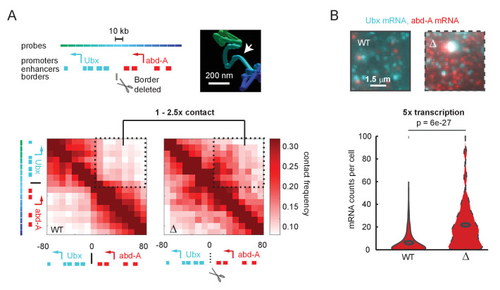
Figure 1. A futile cycle promoter explains super-linear transcriptional responses following subtle changes in enhancer-promoter contact. (A) Quantification of the minor difference in cross-border contact frequency between the Ubx and abd-A regulatory domains in wildtype and domain-border-deleted embryos, quantified by Optical Reconstruction of Chromatin Architecture. (B) Quantification of the major change in transcription of abd-A between wildtype and domain-border-deleted embryos. Raw data taken from Mateo et al., 2019.
Figure 1. A futile cycle promoter explains super-linear transcriptional responses following subtle changes in enhancer-promoter contact. (A) Quantification of the minor difference in cross-border contact frequency between the Ubx and abd-A regulatory domains in wildtype and domain-border-deleted embryos, quantified by Optical Reconstruction of Chromatin Architecture. (B) Quantification of the major change in transcription of abd-A between wildtype and domain-border-deleted embryos. Raw data taken from Mateo et al., 2019.CC BY · PubMed Central
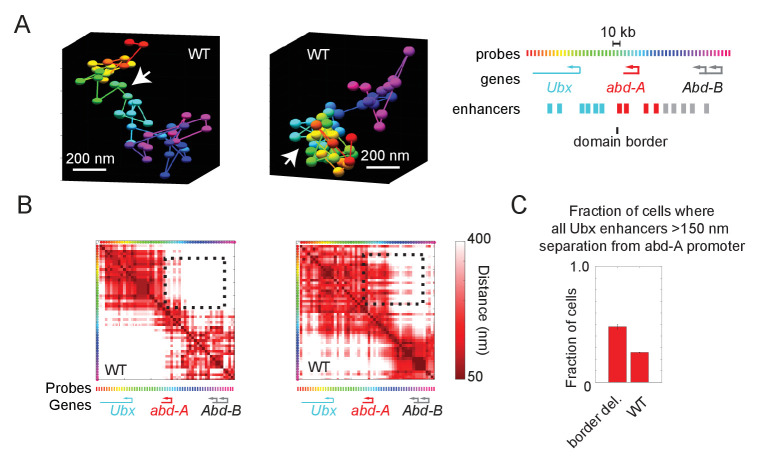
Figure 1—figure supplement 1. Wildtype cells also exhibit cross-border contacts. (A) Images of the Ubx and abd-A domain from two wildtype cells, reconstructed with Optical Reconstruction of Chromatin Architecture. White arrows mark the border between the domains, which are well-separated in the first example and intermixed in the second. (B) Quantification of the respective pairwise distances between all labeled positions along the chromatin for the two cells shown in (A). The black-dotted box highlights the cross-border proximity found in the second cell. (C) Quantification of the frequency in which Ubx enhancers are in proximity to the abd-A promoter in wildtype vs. border-deleted cells.
Figure 1—figure supplement 1. Wildtype cells also exhibit cross-border contacts. (A) Images of the Ubx and abd-A domain from two wildtype cells, reconstructed with Optical Reconstruction of Chromatin Architecture. White arrows mark the border between the domains, which are well-separated in the first example and intermixed in the second. (B) Quantification of the respective pairwise distances between all labeled positions along the chromatin for the two cells shown in (A). The black-dotted box highlights the cross-border proximity found in the second cell. (C) Quantification of the frequency in which Ubx enhancers are in proximity to the abd-A promoter in wildtype vs. border-deleted cells.CC BY · PubMed Central
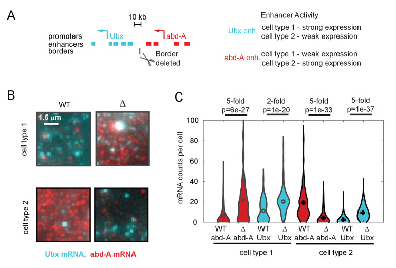
Figure 1—figure supplement 2. Quantitative effects of topologically associated domain (TAD) border deletion on RNA expression. (A) Schematic of the genomic region containing the genes Ubx and abd-A and their surrounding enhancers. Both genes are expressed in two cell types of the abdominal region of the Drosophila embryo, under control of the indicated enhancers. Ubx enhancers drive strong expression in cell type 1 and weak expression in type 2 cells and v.v. for abd-A enhancers, as assayed by both individual enhancer-reporter transgenes and spatial analysis of the domain (Irvine et al., 1991; Mateo et al., 2019; Müller and Bienz, 1991; Qian et al., 1991). The position of the TAD border removed by a 4 kb deletion in ‘border-deleted cells’ is also shown. (B) A zoomed-in view of smRNA fluorescent in situ hybridization signal from single cells of either cell type, showing the typical difference in expression levels in wildtype cells and mutant cells. (C) Quantification of expression levels across the population, shown as a violin plot across all cells. The mRNA type (red = abd-A, cyan = Ubx), genotype (wildtype = solid outline, border-deletion = dotted outline), and cell type are indicated (black = type 1, gray = type 2), along with the median fold change in expression upon border deletion. Results from Wilcoxon comparison of median expression are given as p-values. We note that in cell type 2, abd-A expression decreases in the mutant cells. This decrease in expression is not due to a decrease in contact between abd-A enhancers and abd-A promoter and is likely due to other regulatory mechanisms, as for example, increased contact with silencer elements.
Figure 1—figure supplement 2. Quantitative effects of topologically associated domain (TAD) border deletion on RNA expression. (A) Schematic of the genomic region containing the genes Ubx and abd-A and their surrounding enhancers. Both genes are expressed in two cell types of the abdominal region of the Drosophila embryo, under control of the indicated enhancers. Ubx enhancers drive strong expression in cell type 1 and weak expression in type 2 cells and v.v. for abd-A enhancers, as assayed by both individual enhancer-reporter transgenes and spatial analysis of the domain (Irvine et al., 1991; Mateo et al., 2019; Müller and Bienz, 1991; Qian et al., 1991). The position of the TAD border removed by a 4 kb deletion in ‘border-deleted cells’ is also shown. (B) A zoomed-in view of smRNA fluorescent in situ hybridization signal from single cells of either cell type, showing the typical difference in expression levels in wildtype cells and mutant cells. (C) Quantification of expression levels across the population, shown as a violin plot across all cells. The mRNA type (red = abd-A, cyan = Ubx), genotype (wildtype = solid outline, border-deletion = dotted outline), and cell type are indicated (black = type 1, gray = type 2), along with the median fold change in expression upon border deletion. Results from Wilcoxon comparison of median expression are given as p-values. We note that in cell type 2, abd-A expression decreases in the mutant cells. This decrease in expression is not due to a decrease in contact between abd-A enhancers and abd-A promoter and is likely due to other regulatory mechanisms, as for example, increased contact with silencer elements.CC BY · PubMed Central
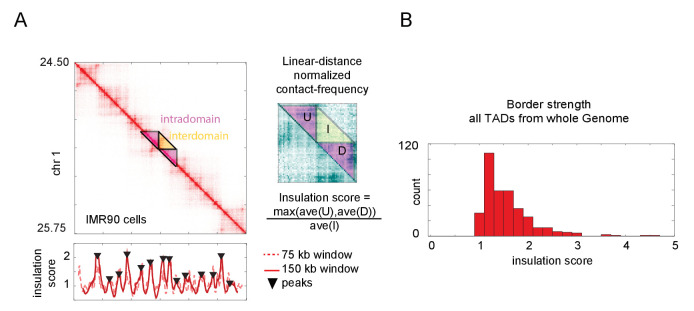
Figure 1—figure supplement 3. Calculation of topologically associated domain (TAD) insulation scores across the genome using Hi-C data. (A) Hi-C data from an arbitrarily selected region of chromosome 1, exhibiting multiple TADs also known as contact domains. The blowout shows a zoomed-in view of the masked region, following normalization to linear-distance separation. The insulation score for this data computed with two different sliding window sizes is plotted below. Peak calls for the 150 kb window are shown, though both windows give similar results. These peaks correspond well to borders of the TADs, as seen by visual inspection. (B) Histogram of the insulation score for all peaks (TAD borders) called genome-wide. The insulation score is normalized for linear distance effects (see Materials and methods), and so reflects the ratio of the preference for intra-TAD vs. inter-TAD contacts.
Figure 1—figure supplement 3. Calculation of topologically associated domain (TAD) insulation scores across the genome using Hi-C data. (A) Hi-C data from an arbitrarily selected region of chromosome 1, exhibiting multiple TADs also known as contact domains. The blowout shows a zoomed-in view of the masked region, following normalization to linear-distance separation. The insulation score for this data computed with two different sliding window sizes is plotted below. Peak calls for the 150 kb window are shown, though both windows give similar results. These peaks correspond well to borders of the TADs, as seen by visual inspection. (B) Histogram of the insulation score for all peaks (TAD borders) called genome-wide. The insulation score is normalized for linear distance effects (see Materials and methods), and so reflects the ratio of the preference for intra-TAD vs. inter-TAD contacts.CC BY · PubMed Central
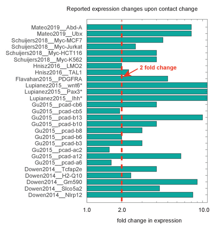
Figure 1—figure supplement 4. Compiled data on fold change in expression following deletion or inversion of topologically associated domain (TAD) borders. Data are organized by source publication, indexed by first author and publication year and gene studied. In some cases, expression was not appreciably detected prior to genomic perturbation, indicated by the asterisk (*). Quantification techniques varied between experiments, and include smFISH, RNAseq, and qPcR. Dotted red line marks genes showing a greater than twofold change.
Figure 1—figure supplement 4. Compiled data on fold change in expression following deletion or inversion of topologically associated domain (TAD) borders. Data are organized by source publication, indexed by first author and publication year and gene studied. In some cases, expression was not appreciably detected prior to genomic perturbation, indicated by the asterisk (*). Quantification techniques varied between experiments, and include smFISH, RNAseq, and qPcR. Dotted red line marks genes showing a greater than twofold change.CC BY · PubMed Central
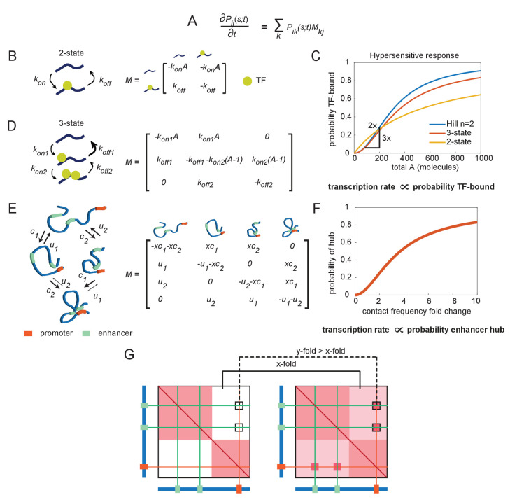
Figure 2. The emergence of hypersensitivity in simple stochastic transcription models. (A) A stochastic model for the evolution of the chemical system, which specifies how the probability of observing the system in state i at time s given it was in state j at time t evolves in time (the forward Kolmogorov equation). M is a transition matrix for the continuous-time Markov system. (B) Cartoon illustration of chemical states for the 2-state enhancer model and the corresponding transition matrix M, as a function of the concentration of transcription factor (TF) activator, A. (C) The probability of TF binding as a function of molecule count, for the2-state and 3-state systems. The Hill equation with a coefficient n = 2 is shown for comparison. (D) As in (B), but for the 3-state enhancer model with two potentially cooperative binding sites. (E) Cartoon depiction of state space for the enhancer cooperativity model and corresponding matrix M for the Markov system/chemical master equation model. The DNA is denoted by a blue polymer, the positions of the enhancers by green segments, and the promoter region by an orange segment. Contacts form with probability c1 and c2 for enhancers 1 and 2, respectively, and separate from loop configuration with probability u1 and u2. (F) Probability of being in the two-loop state as a function of the fold change in loop frequency, for a selection of rate constants chosen to demonstrate the existence of a hypersensitive response. (G) Cartoon depiction of the expected change in contact frequency according to the cooperativity model presented in (E). Enhancer cooperativity leads to the formation of specific loop interactions.
Figure 2. The emergence of hypersensitivity in simple stochastic transcription models. (A) A stochastic model for the evolution of the chemical system, which specifies how the probability of observing the system in state i at time s given it was in state j at time t evolves in time (the forward Kolmogorov equation). M is a transition matrix for the continuous-time Markov system. (B) Cartoon illustration of chemical states for the 2-state enhancer model and the corresponding transition matrix M, as a function of the concentration of transcription factor (TF) activator, A. (C) The probability of TF binding as a function of molecule count, for the2-state and 3-state systems. The Hill equation with a coefficient n = 2 is shown for comparison. (D) As in (B), but for the 3-state enhancer model with two potentially cooperative binding sites. (E) Cartoon depiction of state space for the enhancer cooperativity model and corresponding matrix M for the Markov system/chemical master equation model. The DNA is denoted by a blue polymer, the positions of the enhancers by green segments, and the promoter region by an orange segment. Contacts form with probability c1 and c2 for enhancers 1 and 2, respectively, and separate from loop configuration with probability u1 and u2. (F) Probability of being in the two-loop state as a function of the fold change in loop frequency, for a selection of rate constants chosen to demonstrate the existence of a hypersensitive response. (G) Cartoon depiction of the expected change in contact frequency according to the cooperativity model presented in (E). Enhancer cooperativity leads to the formation of specific loop interactions.CC BY · PubMed Central
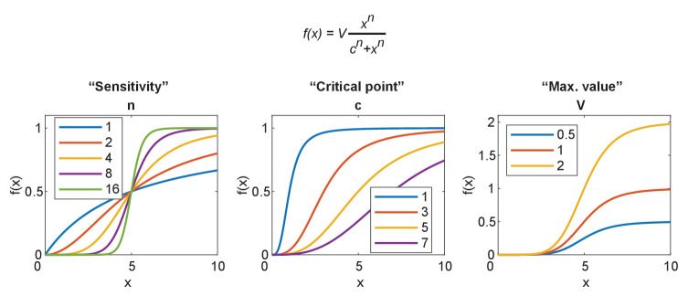
Figure 2—figure supplement 1. Parameterization of the sigmoidal Hill equation. The Hill equation is given at the top. Left: the effect of changing n, which becomes hypersensitive for n > 2 and approaches a digital switch between 0 and v. Center: the effect of changing c, the value at which the function reaches half maximum. Right: the effect of changing v, the maximum value obtained by the function.
Figure 2—figure supplement 1. Parameterization of the sigmoidal Hill equation. The Hill equation is given at the top. Left: the effect of changing n, which becomes hypersensitive for n > 2 and approaches a digital switch between 0 and v. Center: the effect of changing c, the value at which the function reaches half maximum. Right: the effect of changing v, the maximum value obtained by the function.CC BY · PubMed Central
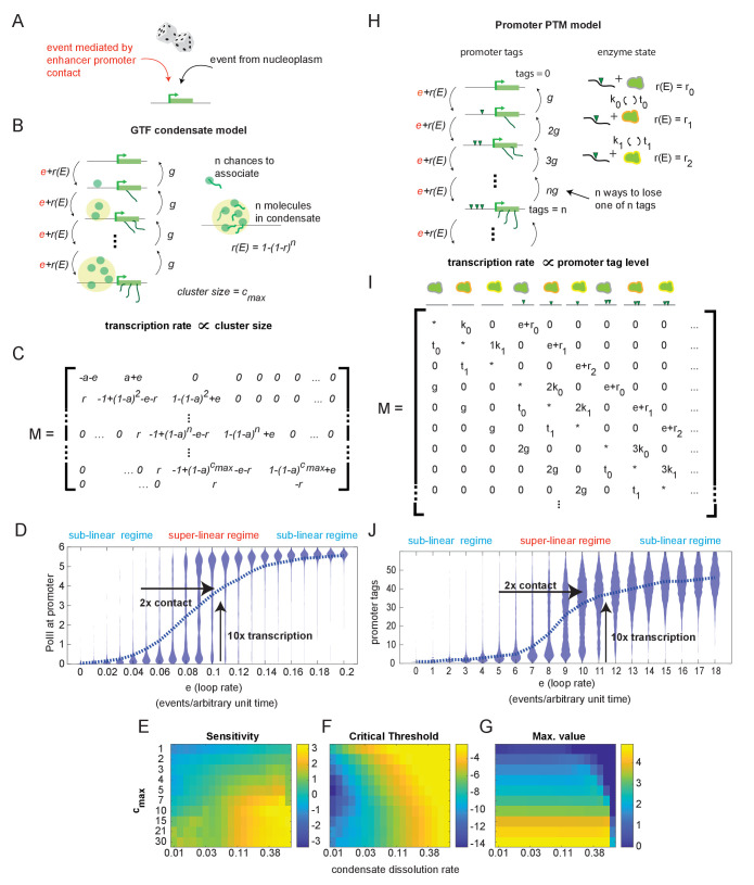
Figure 3. Systems with hypersensitive transcriptional responses to structural perturbation. (A) Generalized cartoon depiction of probabilistic events that affect promoter activity. (B) Schematic of the general transcription factor (GTF) condensate version of the futile cycle model. (C) Markov matrix corresponding to the GTF model version depicted in (B). (D) Simulated condensate size distribution as a function of enhancer-promoter looping rate e. Each violin plot represents a single simulation with fixed e. The superlinear regime reflects where fold change in transcription (linearly proportional to condensate size) is greater than corresponding fold change in e. (E–G) Sensitivity, critical threshold, and maximum value of the GTF system as a function of condensate dissociation rate and max cluster size. (H–J) Same as in (B), (C), and (D), but for the post-translational modification (PTM) model version. Numerical differences in model outputs between D and J, reflect primarily differences in parameter choices rather than intrinsic differences between the model versions, as seen also in the parameter sweeps (E-G, Figure 3—figure supplement 1).
Figure 3. Systems with hypersensitive transcriptional responses to structural perturbation. (A) Generalized cartoon depiction of probabilistic events that affect promoter activity. (B) Schematic of the general transcription factor (GTF) condensate version of the futile cycle model. (C) Markov matrix corresponding to the GTF model version depicted in (B). (D) Simulated condensate size distribution as a function of enhancer-promoter looping rate e. Each violin plot represents a single simulation with fixed e. The superlinear regime reflects where fold change in transcription (linearly proportional to condensate size) is greater than corresponding fold change in e. (E–G) Sensitivity, critical threshold, and maximum value of the GTF system as a function of condensate dissociation rate and max cluster size. (H–J) Same as in (B), (C), and (D), but for the post-translational modification (PTM) model version. Numerical differences in model outputs between D and J, reflect primarily differences in parameter choices rather than intrinsic differences between the model versions, as seen also in the parameter sweeps (E-G, Figure 3—figure supplement 1).CC BY · PubMed Central
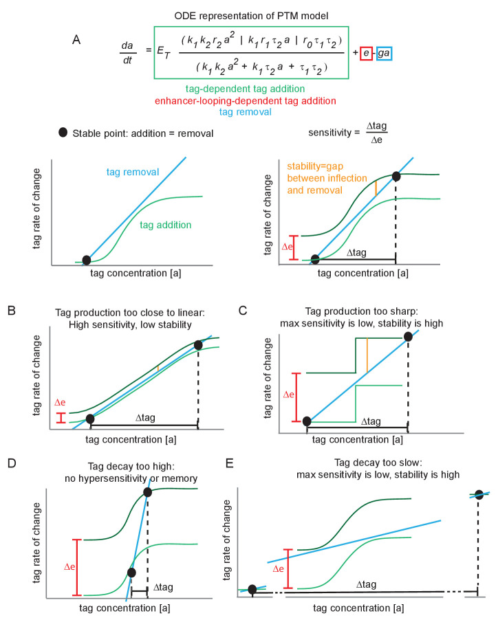
Figure 3—figure supplement 1. Minimal conditions for hypersensitivity in the futile cycle model. (A) Ordinary differential equation representation of the post-translational modification (PTM) model version and corresponding phase portraits for generic parameter values. At a stable point, tag addition and tag removal cancel out, and minor fluctuations about the stable point are pushed back by the imbalance between addition and removal. The sensitivity is defined as the fold change in tag accumulation (proxy for transcription) divided by the fold change in enhancer-promoter (E-P) contact frequency. The stability of a stable point reflects how much of an E-P contact ‘kick’ is needed to jump to the upper stable point. (B) If the tag addition curve is similar to the linear removal curve, the system is highly sensitive to changes in E-P contact but also jumps between stable points very easily (low stability). (C) Under the same reasoning as (B), if the tag addition curve is a step function, the high and low states are highly stable and relatively insensitive to E-P contact changes. (D) If the tag removal curve is steeper than any point on the addition curve, there is only a single stable point that exists for all values of ∆e. This system does not jump between low or high, and is not hypersensitive. (E) Same reasoning as (C).
Figure 3—figure supplement 1. Minimal conditions for hypersensitivity in the futile cycle model. (A) Ordinary differential equation representation of the post-translational modification (PTM) model version and corresponding phase portraits for generic parameter values. At a stable point, tag addition and tag removal cancel out, and minor fluctuations about the stable point are pushed back by the imbalance between addition and removal. The sensitivity is defined as the fold change in tag accumulation (proxy for transcription) divided by the fold change in enhancer-promoter (E-P) contact frequency. The stability of a stable point reflects how much of an E-P contact ‘kick’ is needed to jump to the upper stable point. (B) If the tag addition curve is similar to the linear removal curve, the system is highly sensitive to changes in E-P contact but also jumps between stable points very easily (low stability). (C) Under the same reasoning as (B), if the tag addition curve is a step function, the high and low states are highly stable and relatively insensitive to E-P contact changes. (D) If the tag removal curve is steeper than any point on the addition curve, there is only a single stable point that exists for all values of ∆e. This system does not jump between low or high, and is not hypersensitive. (E) Same reasoning as (C).CC BY · PubMed Central
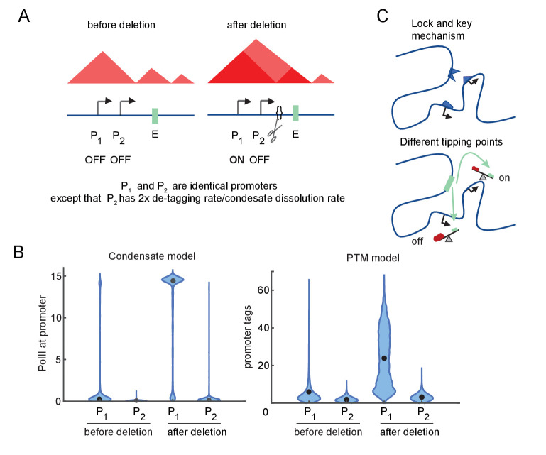
Figure 4. Differential sensitivity to enhancer-promoter (E-P) contact can lead to an illusion of specificity. (A) Cartoon depiction of two simulated promoters undergoing the same change in enhancer contact frequency after a topologically associated domain (TAD)-border deletion. (B) Violin plots of the changes in transcription rates (which are linearly proportional to promoter tag levels) after a twofold increase in the E-P contact rate for each promoter, simulating the border deletion depicted in (A). (C) Cartoon representation of the ‘lock and key’ explanation of E-P specificity, contrasted with the ‘tipping point’ explanation suggested by results in (B).
Figure 4. Differential sensitivity to enhancer-promoter (E-P) contact can lead to an illusion of specificity. (A) Cartoon depiction of two simulated promoters undergoing the same change in enhancer contact frequency after a topologically associated domain (TAD)-border deletion. (B) Violin plots of the changes in transcription rates (which are linearly proportional to promoter tag levels) after a twofold increase in the E-P contact rate for each promoter, simulating the border deletion depicted in (A). (C) Cartoon representation of the ‘lock and key’ explanation of E-P specificity, contrasted with the ‘tipping point’ explanation suggested by results in (B).CC BY · PubMed Central
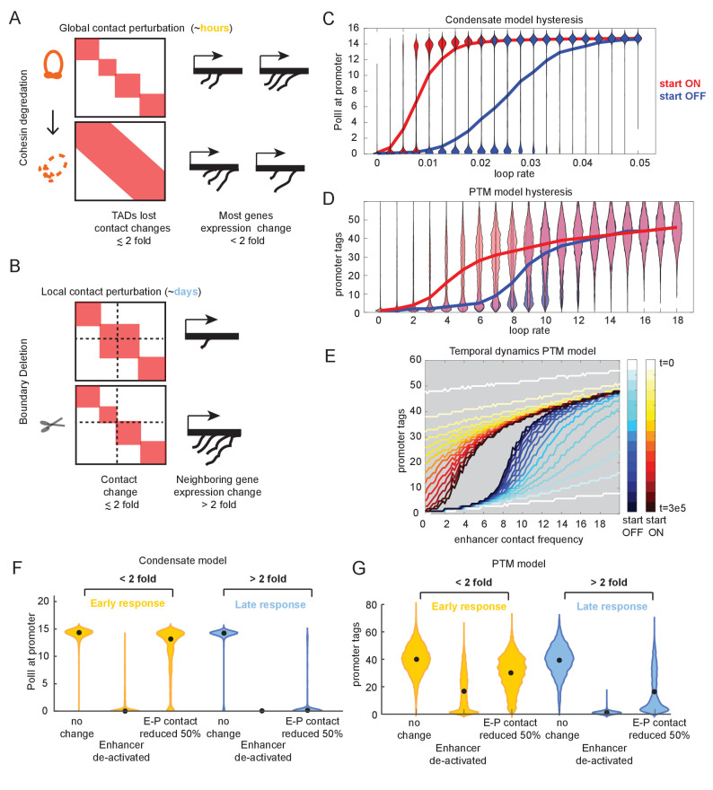
Figure 5. Transcriptional effects of contact perturbation depend on experiment time scale. (A) Schematic of global cohesin loop disruption experiments. (B) Schematic of individual topologically associated domain (TAD) boundary deletion experiments. (C) Violin plots of transcription as a function of enhancer contact, as in Figure 4. Blue and red violin plots represent cell populations that start in the OFF (blue, zero-molecule condensate) or ON state (red, condensate of six molecules). Blue and red lines connect the median behavior from the corresponding simulations. (D) Same as in (C) but for the post-translational modification (PTM) model version (OFF = 0 tags, ON = 30 tags). (E) Median transcription rate for populations starting in ‘OFF’ or ‘ON’ states, observed at different times after initialization of the simulation as indicated by the color legend. (F) Simulation of futile cycle promoter transcription rate as a function of time under different enhancer perturbations for the general transcription factor (GTF) condensate model version. As described in the text, ‘early’ is the amount of time it takes for the promoter to switch off following enhancer deactivation, and late is an order of magnitude or longer later. (G) Same as in (F), but for the PTM model version.
Figure 5. Transcriptional effects of contact perturbation depend on experiment time scale. (A) Schematic of global cohesin loop disruption experiments. (B) Schematic of individual topologically associated domain (TAD) boundary deletion experiments. (C) Violin plots of transcription as a function of enhancer contact, as in Figure 4. Blue and red violin plots represent cell populations that start in the OFF (blue, zero-molecule condensate) or ON state (red, condensate of six molecules). Blue and red lines connect the median behavior from the corresponding simulations. (D) Same as in (C) but for the post-translational modification (PTM) model version (OFF = 0 tags, ON = 30 tags). (E) Median transcription rate for populations starting in ‘OFF’ or ‘ON’ states, observed at different times after initialization of the simulation as indicated by the color legend. (F) Simulation of futile cycle promoter transcription rate as a function of time under different enhancer perturbations for the general transcription factor (GTF) condensate model version. As described in the text, ‘early’ is the amount of time it takes for the promoter to switch off following enhancer deactivation, and late is an order of magnitude or longer later. (G) Same as in (F), but for the PTM model version.CC BY · PubMed Central
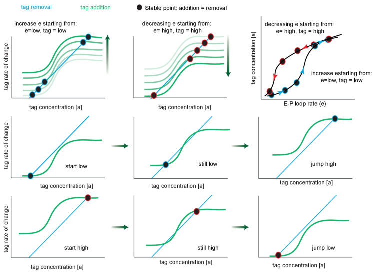
Figure 5—figure supplement 1. Phase portrait exploration of hysteresis. Green curves follow the tag addition rate as a function of tag concentration (sigmoidal), while turquoise plots the tag removal rate (linear). Where these curves intersect (black circles), addition equals removal, representing the steady-state tag concentration of the system, and by proxy, transcription levels. The black points are stable critical points since to the left addition exceeds removal and to the right removal exceeds addition. The fade from white to green (upper left and upper middle) indicates the effect of increasing e, the enhancer-promoter (E-P) loop rate on the position of the stable point, for a system that starts in the low state. Note that after the second step the system has three critical points (crossings points of the removal and addition curves), the system remains in the low state. After the third step, tag addition now exceeds removal at all but the high state, and the system jumps discontinuously to the high state (this is known as a saddle-node bifurcation as the unstable saddle point has collided with the lower stable point). Further increases in e result in only minor further increases. Second and third rows are identical to the white-green fade, but split into multiple panels. Upper right, replotting the stable points on a graph of tag concentration vs. E-P loop rate. The arrows show the effect of increasing (blue) or decreasing (red) e.
Figure 5—figure supplement 1. Phase portrait exploration of hysteresis. Green curves follow the tag addition rate as a function of tag concentration (sigmoidal), while turquoise plots the tag removal rate (linear). Where these curves intersect (black circles), addition equals removal, representing the steady-state tag concentration of the system, and by proxy, transcription levels. The black points are stable critical points since to the left addition exceeds removal and to the right removal exceeds addition. The fade from white to green (upper left and upper middle) indicates the effect of increasing e, the enhancer-promoter (E-P) loop rate on the position of the stable point, for a system that starts in the low state. Note that after the second step the system has three critical points (crossings points of the removal and addition curves), the system remains in the low state. After the third step, tag addition now exceeds removal at all but the high state, and the system jumps discontinuously to the high state (this is known as a saddle-node bifurcation as the unstable saddle point has collided with the lower stable point). Further increases in e result in only minor further increases. Second and third rows are identical to the white-green fade, but split into multiple panels. Upper right, replotting the stable points on a graph of tag concentration vs. E-P loop rate. The arrows show the effect of increasing (blue) or decreasing (red) e.CC BY · PubMed Central
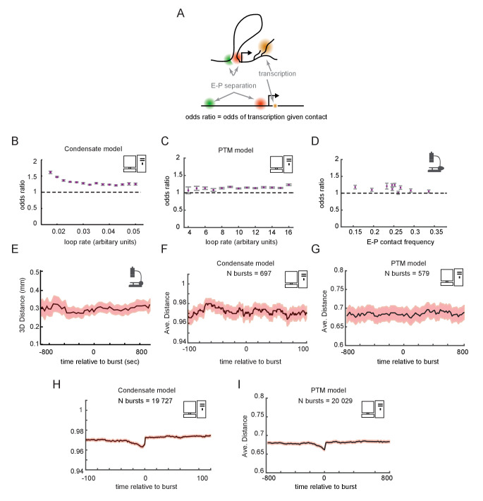
Figure 6. Enhancer-promoter (E-P) contact events may exhibit minimal correlation to transcription events in single cells. (A) Schematic of the textbook expectation of correlation between E-P contact and transcription. (B, C) Odds ratios for observing nascent transcription given E-P proximity, from simulations of the condensate and post-translational modification (PTM) model versions. (D) As in (B) and (C), but for actual data from recent super-resolution imaging experiments (Mateo et al., 2019). Error bars show standard error from bootstrapping. (E) Average measured distance between enhancer and promoter probes relative to the time of transcriptional bursts, reproduced from Figure 6E of Alexander et al., 2019. (F, G) Average E-P distance from simulations of both versions of the futile cycle model, where 0 represents contact and 1 represents no contact, relative to time transcription burst, modeled as a tag concentration > 20. Shaded region denotes ± standard error of the mean. (H, I) As in F and G, with sample size increased to 40-fold.
Figure 6. Enhancer-promoter (E-P) contact events may exhibit minimal correlation to transcription events in single cells. (A) Schematic of the textbook expectation of correlation between E-P contact and transcription. (B, C) Odds ratios for observing nascent transcription given E-P proximity, from simulations of the condensate and post-translational modification (PTM) model versions. (D) As in (B) and (C), but for actual data from recent super-resolution imaging experiments (Mateo et al., 2019). Error bars show standard error from bootstrapping. (E) Average measured distance between enhancer and promoter probes relative to the time of transcriptional bursts, reproduced from Figure 6E of Alexander et al., 2019. (F, G) Average E-P distance from simulations of both versions of the futile cycle model, where 0 represents contact and 1 represents no contact, relative to time transcription burst, modeled as a tag concentration > 20. Shaded region denotes ± standard error of the mean. (H, I) As in F and G, with sample size increased to 40-fold.CC BY · PubMed Central
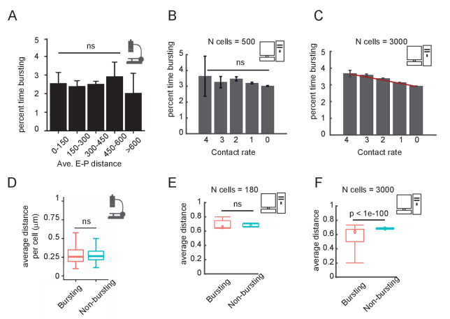
Figure 6—figure supplement 1. Comparison of experimental and simulation results for the post-translational modification (PTM) version of the model on the correlation between enhancer-promoter (E-P) distance and time spent transcribing. (A) Published results from the Sox2 locus (Figure 6C of Alexander et al., 2019), quantifying the percent time spent in the bursting state, for cells binned by average E-P distance. E-P distance is measured using enhancer and promoter probes. (B) Percent time in the bursting transcription state (promoter tag concentration > 20) for simulated cells, binned by observed E-P contact frequency during the simulation window shown. N = 500 cells. Error bars indicate 95% confidence limit around the median. The median time bursting for the high contact sample is not significantly different (ns) from any of the others by a Wilcoxon test (p>0.05). (C) As in (B), but with N = 3000 simulated cells, showing the emergence of a clear and statistically significant trend, Wilcoxon test, p<0.05. Error bars indicate 95% confidence interval. (D) Box-plot analysis taken directly from Figure 6D of Alexander et al., 2019, showing no significant difference in the median distance between bursting and non-bursting promoters. (E) As in (D) but using simulation results sampled in (B). Wilcoxon rank-sum test results indicated by the bar. (F) As in (E) but using simulation results from (C).
Figure 6—figure supplement 1. Comparison of experimental and simulation results for the post-translational modification (PTM) version of the model on the correlation between enhancer-promoter (E-P) distance and time spent transcribing. (A) Published results from the Sox2 locus (Figure 6C of Alexander et al., 2019), quantifying the percent time spent in the bursting state, for cells binned by average E-P distance. E-P distance is measured using enhancer and promoter probes. (B) Percent time in the bursting transcription state (promoter tag concentration > 20) for simulated cells, binned by observed E-P contact frequency during the simulation window shown. N = 500 cells. Error bars indicate 95% confidence limit around the median. The median time bursting for the high contact sample is not significantly different (ns) from any of the others by a Wilcoxon test (p>0.05). (C) As in (B), but with N = 3000 simulated cells, showing the emergence of a clear and statistically significant trend, Wilcoxon test, p<0.05. Error bars indicate 95% confidence interval. (D) Box-plot analysis taken directly from Figure 6D of Alexander et al., 2019, showing no significant difference in the median distance between bursting and non-bursting promoters. (E) As in (D) but using simulation results sampled in (B). Wilcoxon rank-sum test results indicated by the bar. (F) As in (E) but using simulation results from (C).CC BY · PubMed Central

Verification

Claims the paper makes

The claims and statistics of this paper haven’t been checked yet.

Run the check — free, no account needed. It reads the open-access text and checks the sources it cites.

A few free checks a day · papers already verified open instantly · results are public

Claims other papers make about this one

Each is checked against this paper’s own text: does it say what the citing paper says it does?

Self-check

Percentages, sums and reported differences re-computed from the paper’s own numbers.

The self-check needs the paper’s full text.

Citations

Cites

Show all 109 references

Research works printed but not linked: 1

  1. Boettiger AN. 2021. How subtle changes in 3D structure can create large changes in transcription. Software Heritage. swh:1:rev:8af1e7fcf1fa126908465558c4ef6d127000a9c8. https://archive.softwareheritage.org/swh:1:rev:8af1e7fcf1fa126908465558c4ef6d127000a9c8.

Cited by

Sorted by citations

See all 162

Metadata

Authors
Xiao, J. Y., Hafner, A., & Boettiger, A. N.
Affiliations
Stanford University (US)
Corresponding author
Boettiger, Alistair N
Venue
eLife
Published
2021-07-09
Volume
10
ISSN
2050-084X (ISSN-L)
OpenAlex
W3181995425
Cited by
162
References
109
Citations by year
2026: 18 · 2025: 29 · 2024: 37 · 2023: 36 · 2022: 26 · 2021: 16
FWCI
9.10
Type
journal article
Language
en
Open access
Locations
  • eLife (publishedVersion, cc-by)
  • bioRxiv (Cold Spring Harbor Laboratory) (acceptedVersion, cc-by)
  • PubMed Central (publishedVersion, cc-by)
  • PubMed (publishedVersion)
  • DOAJ (DOAJ: Directory of Open Access Journals) (submittedVersion, cc-by-sa)
Funders
  • National Institutes of Health (U01 DK127419)
  • NIH (DGM132935A)
  • Stanford University (GM008294, The Walter V. and Idun Berry Postdoctoral Fellowship Program)
  • Burroughs Wellcome Fund (CASI)
Topics
  • Life Sciences › Biochemistry, Genetics and Molecular Biology › Molecular Biology › Genomics and Chromatin Dynamics
  • Life Sciences › Biochemistry, Genetics and Molecular Biology › Molecular Biology › Gene Regulatory Network Analysis
  • Life Sciences › Biochemistry, Genetics and Molecular Biology › Molecular Biology › Protein Structure and Dynamics
Keywords
topologically associating domains, TAD boundaries, enhancer-promoter interactions, gene expression regulation, bistability, hysteresis, 3D genome organization, stochastic gene expression, promoter activity
MeSH terms
Animals, Chromatin, Gene Expression Regulation, Humans, Hypersensitivity, Promoter Regions, Genetic, Transcription, Genetic, Genome, Computational Biology, Mice

About these checks

Registry, retraction, Cites and statistics results are computed, not judged, with one exception: a printed reference that no index lists is read once by a model before it counts as a citation error. Claims are extracted by a model and kept only when their quote appears verbatim in the text; each cited source is then checked, with a model’s help, for whether it says what the claim relies on. Those verdicts can be wrong — read the claim’s quote and the cited source before relying on one.

Statistics and arithmetic are recomputed, not judged.

Confidence bands are shown only for fields calibrated on our annotated test set. None is calibrated yet, so no band is shown.

What counts as a claim ›How we measure confidence ›How we check this ›

Are you an author, or do you see a problem with this page? Request a review