

Passive exposure to task-relevant stimuli enhances categorization learning
Open accessPublished version of a preprint
The DOI matches its Crossref record; 41 of the 42 references it cites were found in a registry or an index; none of the 11 sources its claims cite is checked for support yet.
Abstract
Learning to perform a perceptual decision task is generally achieved through sessions of effortful practice with feedback. Here, we investigated how passive exposure to task-relevant stimuli, which is relatively effortless and does not require feedback, influences active learning. First, we trained mice in a sound-categorization task with various schedules combining passive exposure and active training. Mice that received passive exposure exhibited faster learning, regardless of whether this exposure occurred entirely before active training or was interleaved between active sessions. We next trained neural-network models with different architectures and learning rules to perform the task. Networks that use the statistical properties of stimuli to enhance separability of the data via unsupervised learning during passive exposure provided the best account of the behavioral observations. We further found that, during interleaved schedules, there is an increased alignment between weight updates from passive exposure and active training, such that a few interleaved sessions can be as effective as schedules with long periods of passive exposure before active training, consistent with our behavioral observations. These results provide key insights for the design of efficient training schedules that combine active learning and passive exposure in both natural and artificial systems.
Overview
CoChat Summary
TL;DR
Passive exposure to task-relevant frequency-modulated sounds sped up sound-categorization learning in adult mice whether it occurred before or interleaved with active training. Neural-network models suggest this benefit arises when unsupervised learning in early layers builds latent representations that supervised readout can use, with interleaved schedules aligning active and passive weight updates.
Key findings
- Mice with passive exposure learned faster than active-only mice: time to 70% correct was shorter (p=0.01 for A only vs A+P; p=0.006 for A only vs P:A; p=0.71 for A+P vs P:A, Wilcoxon rank-sum test), and estimated performance at 21 days was higher (p=0.01, p=0.006, p=0.47 respectively). Last-4-day S3 performance matched these comparisons (p=0.01, p=0.006, p=0.71).
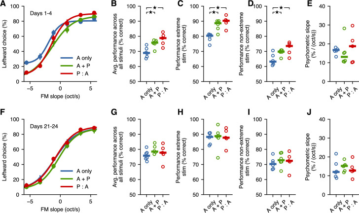
- Passive exposure also improved psychometric performance in S4, including intermediate sounds not used in S3: overall performance p=0.01 for A only vs A+P, p=0.01 for A only vs P:A, p=0.27 for A+P vs P:A; intermediate stimuli p=0.037, p=0.028, p=0.36; psychometric slopes did not differ significantly (p=0.07, p=1, p=0.86). After 21 days of S4, A-only mice improved (p=0.031) and all cohorts became indistinguishable (p>0.26).
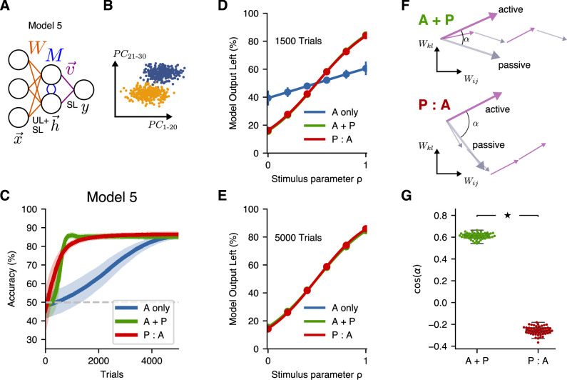
- In models, a one-layer model did not benefit from passive pre-exposure; two-layer models with unsupervised learning in the first layer and supervised learning at readout accounted for faster learning with passive exposure. Model 5, combining supervised and unsupervised learning at the input layer, reproduced similar A+P and P:A benefits and psychometric curves; active and passive weight updates were more aligned for A+P than P:A (p<10⁻³, Wilcoxon rank-sum test).
Methods
- 27 wild-type C57BL/6J adult mice (both sexes, 2.5–4 months) were water-restricted and trained on a two-alternative choice task to discriminate positive vs negative slopes of 200-ms frequency-modulated sounds; cohorts were A only (8 mice), A+P (9), P:A (9), with one mouse excluded. Passive exposure consisted of ~3600 trials/day (600 presentations of each of six stimuli, every 4.5 s) in home cages.
- Behavioral analysis fit a straight line to daily S3 performance to estimate 21-day performance and days to 70% correct; Gaussian mixture models tested bimodality; psychometric curves were sigmoidal fits; cohort comparisons used Wilcoxon rank-sum tests.
- Neural-network models were implemented in JAX with five architectures/learning rules; schedules were A only (5000 active trials), A+P (5000 active trials each followed by 9 passive exposures), and P:A (45,000 passive exposures then 5000 active trials), using isotropic, non-isotropic, and non-aligned input distributions.
Limitations
- The paper states that its modeling approach omits features that may be important for fully capturing unsupervised learning during passive exposure in the brain; more sophisticated approaches beyond linear dimensionality reduction will be required when relevant stimulus features are encoded nonlinearly, as likely for natural sounds.
- The paper states that the comparable benefits of P:A and A+P could be a consequence of the large number of daily passive-exposure trials, and that a comprehensive evaluation of learning performance as a function of passive-exposure number is needed; models most often found pre-exposure led to larger gains (Models 3 and 4), though Model 5 did not.
- Evident from the text: the study is limited to one auditory categorization task in mice, with no neural recordings, and the slow-learner comparisons were not statistically significant (p-values 0.064–0.16); the models use simplified linear networks and specific stimulus distributions.
Model-written summary. Check it against the paper before relying on it.
Integrity signals
Registry
Cites
Statistics
Figures




Verification
Claims the paper makes
0 Valid · 0 Not valid · 7 Not checked · 55 Own results and interpretations
A result the paper reports from its own data — it cites no other source for it, so there is none to check. The quote shows it is in the paper.
In the paper
“while we found no statistically significant difference between the A + P and P:A cohorts (p=0.71, Wilcoxon rank-sum test).”
§ Passive exposure to task-relevant stimuli enhances categorization learning > Results > Passive exposure to sounds improves learning
plain- Asserted: passes — The authors put it forward as true.
- Checkable: passes — It can be checked against evidence.
- Load-bearing: passes — The paper’s conclusions depend on it.
- Based: passes — The paper gives a reason why it holds.
A result the paper reports from its own data — it cites no other source for it, so there is none to check. The quote shows it is in the paper.
In the paper
“This disparity in overall performance was the result of differences in both the responses to the extreme sounds (Figure 3C) as well the responses to intermediate sounds (p=0.037 for A only vs. A + P, p=0.028 for A only vs. P:A, p=0.36 for A + P vs. P:A, Wilcoxon rank-sum test) (Figure 3D).”
§ Passive exposure to task-relevant stimuli enhances categorization learning > Results > Passive exposure influences responses to intermediate sounds not used during training
plainstates a cause- Asserted: passes — The authors put it forward as true.
- Checkable: passes — It can be checked against evidence.
- Load-bearing: passes — The paper’s conclusions depend on it.
- Based: passes — The paper gives a reason why it holds.
A result the paper reports from its own data — it cites no other source for it, so there is none to check. The quote shows it is in the paper.
In the paper
“Comparisons across cohorts matched those observed from the linear fit estimates, where mice with passive exposure displayed higher performance (p=0.01 for A only vs. A + P, p=0.006 for A only vs. P:A, p=0.71 for A + P vs. P:A, Wilcoxon rank-sum test).”
§ Passive exposure to task-relevant stimuli enhances categorization learning > Results > Passive exposure to sounds improves learning
plainstates an association- Asserted: passes — The authors put it forward as true.
- Checkable: passes — It can be checked against evidence.
- Load-bearing: passes — The paper’s conclusions depend on it.
- Based: passes — The paper gives a reason why it holds.
A result the paper reports from its own data — it cites no other source for it, so there is none to check. The quote shows it is in the paper.
In the paper
“Mice that received passive exposure exhibited faster learning, regardless of whether this exposure occurred entirely before active training or was interleaved between active sessions.”
- Also stated in: § Passive exposure to sounds improves learning · hedged
“Overall, these results indicate that passive exposure to task-relevant sounds—either before or during learning—can enhance acoustic categorization learning in adult mice, and they point to a non-trivial interaction between passive exposure and active learning, which we further investigate in our theoretical analysis below.”
- Also stated in: § Introduction · plain
“We found that passive presentation of stimuli enhanced learning speed in mice, either when passive presentation occurred before any active training or when passive-exposure sessions were interleaved with active training.”
§ Passive exposure to task-relevant stimuli enhances categorization learning > Abstract
plainstates a cause- Asserted: passes — The authors put it forward as true.
- Checkable: passes — It can be checked against evidence.
- Load-bearing: passes — The paper’s conclusions depend on it.
- Based: passes — The paper gives a reason why it holds.
- Also stated in: § Passive exposure to sounds improves learning · hedged
A result the paper reports from its own data — it cites no other source for it, so there is none to check. The quote shows it is in the paper.
In the paper
“while we found no difference between the A + P and P:A cohorts (p=0.47, Wilcoxon rank-sum test).”
§ Passive exposure to task-relevant stimuli enhances categorization learning > Results > Passive exposure to sounds improves learning
plain- Asserted: passes — The authors put it forward as true.
- Checkable: passes — It can be checked against evidence.
- Load-bearing: passes — The paper’s conclusions depend on it.
- Based: passes — The paper gives a reason why it holds.
28 more claims
Create a free account to see all 62 claims and to verify the 10 references still open.
- It may state two separate claims as one. 16
- Probably not a substantial claim. 15
Self-check
Percentages, sums and reported differences re-computed from the paper’s own numbers.
Each contradiction between two passages listed here was confirmed by an independent check.
Rated major: it would touch a result — a value a result rests on, reported and recomputed p-values on opposite sides of the significance level, two passages that conflict with no sign which is right, or a cited work retracted before this paper was published.
In the paper
§ Passive exposure to task-relevant stimuli enhances categorization learning > Results > Building higher-dimensional latent representations improves learning for more-general input distributions
“We set the extreme means ±μ→0=±e→2, where e→i is the unit vector along the ith dimension. For these inputs, the coding direction represents the second principal component (Figure 6A).”
§ Passive exposure to task-relevant stimuli enhances categorization learning > Methods > Modeling
“For the non-isotropic input, we set d=50 and μ→0=1.4e→2, and the covariance to Σ=diag(σ1²,σ2²,σ2²,…), with σ1=1 and σ2=√8.”
Rated minor: it would not touch a result — a value no result rests on, a p-value that stays on the same side of the significance level, or a conflict that is clerical, resolved elsewhere in the paper, or outside its own findings.
In the paper
§ Passive exposure to task-relevant stimuli enhances categorization learning > Results > Passive exposure is beneficial when building latent representations with unsupervised learning
“The output of the model was then S(v→⋅Wh→).”
§ Passive exposure to task-relevant stimuli enhances categorization learning > Methods > Modeling
“The two-layer architecture introduces additional weights W to map the input x→ to a latent representation h→=Wx→, which is used by the readout weights v→ to produce the output y^=S(v→⋅Wx→).”
Rated minor: it would not touch a result — a value no result rests on, a p-value that stays on the same side of the significance level, or a conflict that is clerical, resolved elsewhere in the paper, or outside its own findings.
In the paper
§ Passive exposure to task-relevant stimuli enhances categorization learning > Results > Passive exposure influences responses to intermediate sounds not used during training
“We first estimated the average psychometric curves across all mice from each cohort during the first 4 days of S4 (Figure 3A).”
§ Passive exposure to task-relevant stimuli enhances categorization learning > Results > Passive exposure influences responses to intermediate sounds not used during training
“(A) Average psychometric performance for the first 4 days of stage S4 across fast learners from each group.”
Citations
Cites
BERT: Pre-training of Deep Bidirectional Transformers for Language Understanding
Devlin, J., Chang, M.-W., Lee, K., & Toutanova, K. (2018) · arXiv · doi:10.48550/arxiv.1810.04805 · Cited by 73,173
Scikit-learn: Machine Learning in Python
Pedregosa, F., Varoquaux, G., Gramfort, A., Michel, V., Thirion, B., Grisel, O., Blondel, M., Müller, A., Nothman, J., Louppe, G., et al. (2012) · arXiv · doi:10.48550/arxiv.1201.0490 · Cited by 71,016
Scikit-learn: Machine Learning in Python
(2011) · Journal of Machine Learning Research · doi:10.5555/1953048.2078195 · Cited by 8,539
Representation Learning with Contrastive Predictive Coding
Oord, A. V. D., Li, Y., & Vinyals, O. (2018) · arXiv · doi:10.48550/arxiv.1807.03748 · Cited by 6,242
wav2vec 2.0: A Framework for Self-Supervised Learning of Speech Representations
Baevski, A., Zhou, Y., Mohamed, A., & Auli, M. (2020) · neural information processing systems · Cited by 5,822
Bootstrap Your Own Latent: A New Approach to Self-Supervised Learning
Grill, J.-B., Strub, F., Altché, F., Tallec, C., Richemond, P. H., Buchatskaya, E., Doersch, C., Pires, B. A., Guo, Z. D., Azar, M. G., et al. (2020) · arXiv · doi:10.48550/arxiv.2006.07733 · Cited by 3,846
A survey on semi-supervised learning
van Engelen, J. E., & Hoos, H. H. (2020) · Machine Learning · doi:10.1007/s10994-019-05855-6 · Cited by 2,666
wav2vec 2.0: A Framework for Self-Supervised Learning of Speech Representations
Baevski, A., Zhou, H., Mohamed, A., & Auli, M. (2020) · arXiv · doi:10.48550/arxiv.2006.11477 · Cited by 2,369
Simplified neuron model as a principal component analyzer
Oja, E. (1982) · Journal of Mathematical Biology · doi:10.1007/bf00275687 · Cited by 2,309
Infant sensitivity to distributional information can affect phonetic discrimination
Maye, J., Werker, J. F., & Gerken, L. (2002) · Cognition · doi:10.1016/s0010-0277(01)00157-3 · Cited by 1,364
Hensch, T. K. (2004) · Annual Review of Neuroscience · doi:10.1146/annurev.neuro.27.070203.144327 · Cited by 1,300 · cited 1×
“Multiple studies have demonstrated that the statistics of sensory stimulation during an animal’s development have a strong influence on the perceptual abilities (and associated neural correlates) in the adult ( Hensch, 2004 ).”
BackgroundKuhl, P. K., Tsao, F.-M., & Liu, H.-M. (2003) · Proceedings of the National Academy of Sciences · doi:10.1073/pnas.1532872100 · Cited by 1,237
Simulation physiologischer Regelkreise mit der objektorientierten Modellbibliothek “HumanLib”
Brunberg, A., Spillner, J., Autschbach, R., & Abel, D. (2011) · auto · doi:10.1524/auto.2011.0951 · Cited by 1,008
Self-labeled techniques for semi-supervised learning: taxonomy, software and empirical study
Triguero, I., García, S., & Herrera, F. (2015) · Knowledge and Information Systems · doi:10.1007/s10115-013-0706-y · Cited by 573
Perceptual Learning Directs Auditory Cortical Map Reorganization through Top-Down Influences
Polley, D. B., Steinberg, E. E., & Merzenich, M. M. (2006) · The Journal of Neuroscience · doi:10.1523/jneurosci.3771-05.2006 · Cited by 551
Neural population coding of sound level adapts to stimulus statistics
Dean, I., Harper, N. S., & McAlpine, D. (2005) · Nature Neuroscience · doi:10.1038/nn1541 · Cited by 516
Adaptive coding of visual information in neural populations
Gutnisky, D. A., & Dragoi, V. (2008) · Nature · doi:10.1038/nature06563 · Cited by 337
Belkin, M., Niyogi, P., & Sindhwani, V. (2005) · Cited by 323
Adaptive filtering enhances information transmission in visual cortex
Sharpee, T. O., Sugihara, H., Kurgansky, A. V., Rebrik, S. P., Stryker, M. P., & Miller, K. D. (2006) · Nature · doi:10.1038/nature04519 · Cited by 311
Auditory critical periods: A review from system’s perspective
Kral, A. (2013) · Neuroscience · doi:10.1016/j.neuroscience.2013.05.021 · Cited by 304
Temporal plasticity in the primary auditory cortex induced by operant perceptual learning
Bao, S., Chang, E. F., Woods, J., & Merzenich, M. M. (2004) · Nature Neuroscience · doi:10.1038/nn1293 · Cited by 265
McLaren, I. P. L., Kaye, H., & Mackintosh, N. J. (1989) · Cited by 264
Naturalistic experience transforms sensory maps in the adult cortex of caged animals
Polley, D. B., Kvašňák, E., & Frostig, R. D. (2004) · Nature · doi:10.1038/nature02469 · Cited by 204
Environmental enrichment and the sensory brain: The role of enrichment in remediating brain injury
Alwis, D. S., & Rajan, R. (2014) · Frontiers in Systems Neuroscience · doi:10.3389/fnsys.2014.00156 · Cited by 129
Top-down modulation of sensory cortex gates perceptual learning
Caras, M. L., & Sanes, D. H. (2017) · Proceedings of the National Academy of Sciences · doi:10.1073/pnas.1712305114 · Cited by 124
Pehlevan, C., Hu, T., & Chklovskii, D. B. (2015) · Neural Computation · doi:10.1162/neco_a_00745 · Cited by 98
Frequency Tuning in the Behaving Mouse: Different Bandwidths for Discrimination and Generalization
de Hoz, L., & Nelken, I. (2014) · PLoS ONE · doi:10.1371/journal.pone.0091676 · Cited by 78
Olfactory enrichment improves the recognition of individual components in mixtures
Mandairon, N., Stack, C. M., & Linster, C. (2006) · Physiology & Behavior · doi:10.1016/j.physbeh.2006.07.013 · Cited by 77
Gold, J. I., & Watanabe, T. (2010) · Current Biology · doi:10.1016/j.cub.2009.10.066 · Cited by 71
Shifting and scaling adaptation to dynamic stimuli in somatosensory cortex
Garcia‐Lazaro, J. A., Ho, S. S. M., Nair, A., & Schnupp, J. W. H. (2007) · European Journal of Neuroscience · doi:10.1111/j.1460-9568.2007.05847.x · Cited by 44
Wright, B. A., Baese-Berk, M. M., Marrone, N., & Bradlow, A. R. (2015) · The Journal of the Acoustical Society of America · doi:10.1121/1.4927411 · Cited by 32
Self-citationNoise correlations for faster and more robust learning
Nassar, M. R., Scott, D., & Bhandari, A. (2021) · The Journal of Neuroscience · doi:10.1523/jneurosci.3045-20.2021 · Cited by 28
Incidental auditory category learning
Gabay, Y., Dick, F. K., Zevin, J. D., & Holt, L. L. (2015) · Journal of Experimental Psychology: Human Perception and Performance · doi:10.1037/xhp0000073 · Cited by 26
Incidental auditory category learning
Holt, L. L., Gabay, Y., Dick, F., & Zevin, J. D. (2015) · The Journal of the Acoustical Society of America · doi:10.1121/1.4920684 · Cited by 12
Fleming, G., Wright, B. A., & Wilson, D. A. (2019) · Chemical Senses · doi:10.1093/chemse/bjy083 · Cited by 12
Meta-Learning Biologically Plausible Semi-Supervised Update RulesPreprint
Gu, K., Greydanus, S., Metz, L., Maheswaranathan, N., & Sohl‐Dickstein, J. (2019) · bioRxiv (Cold Spring Harbor Laboratory) · doi:10.1101/2019.12.30.891184 · Cited by 12
Contextual Integration in Cortical and Convolutional Neural Networks
Iyer, R., Hu, B., & Mihalaş, Ş. (2020) · Frontiers in Computational Neuroscience · doi:10.3389/fncom.2020.00031 · Cited by 10
Holland, P. C. (2017) · Learning & Behavior · doi:10.3758/s13420-017-0297-7 · Cited by 8
A Neural Network for Semi-supervised Learning on Manifolds
Genkin, A., Sengupta, A. M., & Chklovskii, D. B. (2019) · Lecture notes in computer science · doi:10.1007/978-3-030-30487-4_30 · Cited by 8
Schmid, C., Haziq, M., Baese‐Berk, M. M., Murray, J. M., & Jaramillo, S. (2023) · Zenodo (CERN European Organization for Nuclear Research) · doi:10.5281/zenodo.10360066 · Cited by 2
Self-citationUnsupervised Speech Recognition
Baevski, A., Hsu, W.-N., Conneau, A., & Auli, M. (2021) · arXiv · doi:10.48550/arxiv.2105.11084
Research works printed but not linked: 1
- Schmid C. 2023. Behaviour-models. Software Heritage. swh:1:rev:bdf55cd53c845fe00b7bc62476584f4eab1abc66. https://archive.softwareheritage.org/swh:1:dir:7fa425b87271bd779b361ea0a1d92ee699db85c7;origin=https://github.com/cschmidat/behaviour-models;visit=swh:1:snp:92c05cc5e8af3e633686e4f5c2417940a2417e14;anchor=swh:1:rev:bdf55cd53c845fe00b7bc62476584f4eab1abc66.
Cited by
Cortical reactivations predict future sensory responses
Nguyen, N. D., Lutas, A., Amsalem, O., Fernando, J., Ahn, A. Y.-E., Hakim, R., Vergara, J., McMahon, J., Dimidschstein, J., Sabatini, B. L., et al. (2023) · Nature · doi:10.1038/s41586-023-06810-1 · Cited by 55
Demystifying unsupervised learning: how it helps and hurts
Bröker, F., Holt, L. L., Roads, B. D., Dayan, P., & Love, B. C. (2024) · Trends in Cognitive Sciences · doi:10.1016/j.tics.2024.09.005 · Cited by 36
Neural Correlates of Category Learning in Monkey Inferior Temporal Cortex
Pearl, J. E., Matsumoto, N., Hayashi, K., Matsuda, K., Miura, K., Nagai, Y., Miyakawa, N., Minamimoto, T., Saunders, R. C., Sugase-Miyamoto, Y., et al. (2024) · Journal of Neuroscience · doi:10.1523/jneurosci.0312-24.2024 · Cited by 10
A corticostriatal learning mechanism linking excess striatal dopamine and auditory hallucinationsPreprint
Lakshminarasimhan, K. J., Buck, J., Kellendonk, C., & Horga, G. (2025) · bioRxiv (Cold Spring Harbor Laboratory) · doi:10.1101/2025.03.18.643990 · Cited by 6
A cortical output channel for perceptual categorization
Schneider, N. A., Malina, M., & Williamson, R. S. (2026) · Science Advances · doi:10.1126/sciadv.aef3715 · Cited by 4
Metadata
- Authors
- Schmid, C., Haziq, M., Baese-Berk, M. M., Murray, J. M., & Jaramillo, S.
- Affiliations
- University of Oregon (US)
- Department of Linguistics, University of Oregon
- Corresponding author
- Murray, James M
- Jaramillo, Santiago
- Venue
- eLife
- Publisher
- eLife Sciences Publications, Ltd
- Published
- 2024-01-24
- Volume
- 12
- ISSN
- 2050-084X (ISSN-L)
- PMC
- PMC10945695
- OpenAlex
- W4385066317
- Cited by
- 6
- References
- 42
- Citations by year
- 2026: 1 · 2025: 2 · 2024: 2
- FWCI
- 0.63
- Type
- journal article
- Language
- en
- Open access
- gold
- doi.org
- Licence
- cc-by
- creativecommons.org/licenses/by/4.0/ (vor)
- creativecommons.org/licenses/by/4.0/ (am)
- creativecommons.org/licenses/by/4.0/ (tdm)
- Locations
- eLife (publishedVersion, cc-by)
- eLife (submittedVersion, cc-by)
- bioRxiv (Cold Spring Harbor Laboratory) (submittedVersion, cc-by-nc)
- PubMed Central (publishedVersion, cc-by)
- PubMed (publishedVersion)
- PubMed Central (submittedVersion, cc-by-nc)
- PubMed (submittedVersion)
- DOAJ (DOAJ: Directory of Open Access Journals) (submittedVersion, cc-by-sa)
- Funders
- National Science Foundation (2024926)
- National Institute of Neurological Disorders and Stroke (Pathway to Independence Award R00NS114194, R01NS118461)
- University of Oregon (Office of the Vice President for Research & Innovation I3 award)
- Topics
- Life Sciences › Neuroscience › Cognitive Neuroscience › Memory and Neural Mechanisms
- Physical Sciences › Computer Science › Artificial Intelligence › Domain Adaptation and Few-Shot Learning
- Physical Sciences › Computer Science › Artificial Intelligence › Machine Learning and Algorithms
- Keywords
- passive exposure, category learning, perceptual decision making, unsupervised learning, audio classification, neural network model, weight updating, mice
- MeSH terms
- Behavior Observation Techniques, Animals, Sound, Neural Networks, Computer, Mice
About these checks
Registry, retraction, Cites and statistics results are computed, not judged, with one exception: a printed reference that no index lists is read once by a model before it counts as a citation error. Claims are extracted by a model and kept only when their quote appears verbatim in the text; each cited source is then checked, with a model’s help, for whether it says what the claim relies on. Those verdicts can be wrong — read the claim’s quote and the cited source before relying on one.
A language model drew the claims from the paper on 2026-11-19, under version 3 of the claim definition (model deepseek-v4.1-flash, prompt extract-v3).
A second model labelled each claim on 2026-11-19 (model jev-1.13-20260917, definition revision gold-guideline-v0.2).
Statistics and arithmetic are recomputed, not judged.
Confidence bands are shown only for fields calibrated on our annotated test set. None is calibrated yet, so no band is shown.
What counts as a claim ›How we measure confidence ›How we check this ›
Are you an author, or do you see a problem with this page? Request a review
Data sources
Bibliographic data: Semantic Scholar, OpenAlex, Crossref.
Contains information from the Semantic Scholar Academic Graph Datasets, made available under the ODC Attribution License (ODC-BY 1.0).
Semantic Scholar’s data is described in: Kinney, R., et al. (2023). The Semantic Scholar Open Data Platform. arXiv:2301.10140.
