

The DOI matches its Crossref record; 3 of the 3 references it cites were found in a registry or an index.
Tailoring Ultra‐High‐Order Optical Skyrmions
Abstract
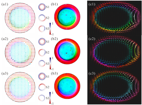
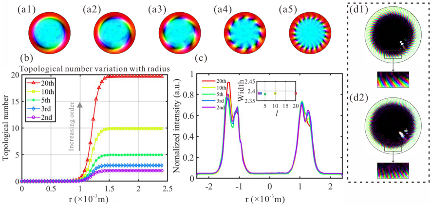
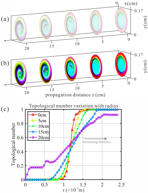
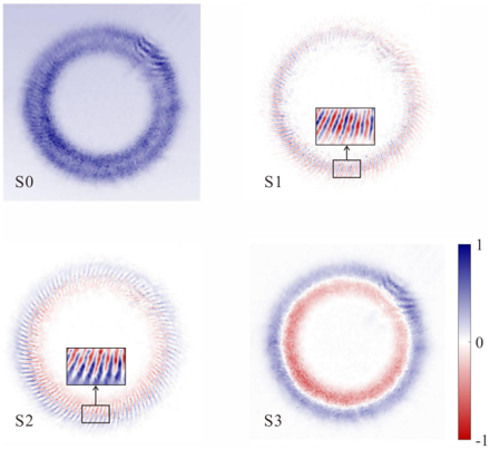
As quasiparticles with topological spin textures, skyrmions have drawn considerable interest from the condensed matter and structured wave communities, offering potential for next‐generation high‐density, robust information technologies. Nevertheless, generating high‐order skyrmions remains a significant challenge, as they have not been reliably observed in any physical system. Here, the method is proposed to create and control ultra‐high‐order skyrmions (skyrmion number up to 400 th ) in a structured light system. The topological state transition between bimerons and skyrmions is also experimentally controlled, the transverse size of an arbitrary‐order skyrmionic beam is tailored independently of the topological number, and ensure the topological stability upon propagation. This work provides solutions for topologically resilient communication and memory, significantly enhancing information capacity.
Overview
The claims and statistics of this paper haven’t been checked yet.
Run the check — free, no account needed. It reads the open-access text and checks the sources it cites.
Integrity signals
Registry
Cites
Statistics
Figures
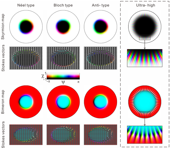
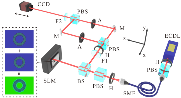
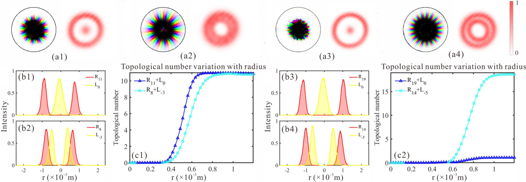
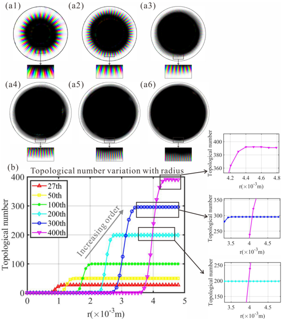
Verification
Claims the paper makes
The claims and statistics of this paper haven’t been checked yet.
Run the check — free, no account needed. It reads the open-access text and checks the sources it cites.
Claims other papers make about this one
Each is checked against this paper’s own text: does it say what the citing paper says it does?
In the citing paper
“as has been shown recently (82), whose transverse intensity distribution is independent of the topological charge.”
From Topological robustness of optical skyrmions through a real-world free-space link (2026) · cites this paper as [82]
Self-check
Percentages, sums and reported differences re-computed from the paper’s own numbers.
The self-check needs the paper’s full text.
Citations
Cites
Optical skyrmion lattice in evanescent electromagnetic fields
Tsesses, S., Ostrovsky, E., Cohen, K., Gjonaj, B., Lindner, N. H., & Bartal, G. (2018) · Science · doi:10.1126/science.aau0227 · Cited by 514
Optical skyrmions and other topological quasiparticles of light
Shen, Y., Zhang, Q., Shi, P., Du, L., Yuan, X., & Zayats, A. V. (2024) · Nature Photonics · doi:10.1038/s41566-023-01325-7 · Cited by 469
Self-citationGeneration of Optical Skyrmions with Tunable Topological Textures
Shen, Y., Martínez, E. C., & Rosales-Guzmán, C. (2022) · ACS Photonics · doi:10.1021/acsphotonics.1c01703 · Cited by 278
Self-citation
Research works printed but not linked: 55
- 10.1016/0029-5582(62)90775-7 · DOI
- 10.1126/science.1166767 · DOI
- 10.1038/nature09124 · DOI
- 10.1038/s42254-020-0203-7 · DOI
- 10.1126/sciadv.adj9373 · DOI
- 10.1038/nmat4223 · DOI
- 10.1038/natrevmats.2017.31 · DOI
- 10.1038/s41467-019-14095-0 · DOI
- 10.1038/s41586-018-0745-3 · DOI · Paper page
- 10.1038/s41524-020-00435-y · DOI
- 10.1038/s41567-019-0476-x · DOI
- 10.1038/s41565-021-00954-9 · DOI · Paper page
- 10.1038/s41467-021-21250-z · DOI · Paper page
- 10.1103/PhysRevB.107.195428 · DOI
- 10.1038/s41567-019-0487-7 · DOI · Paper page
- 10.1515/nanoph-2023-0741 · DOI
- 10.1002/lpor.202300155 · DOI · Paper page
- 10.1364/OL.431122 · DOI · Paper page
- 10.1002/adpr.202200350 · DOI
- 10.1364/AOP.547634 · DOI
- 10.1063/5.0265736 · DOI
- 10.1038/s41566-019-0538-8 · DOI
- 10.1063/5.0192239 · DOI
- 10.1364/PRJ.499485 · DOI
- 10.1364/OPTICA.540469 · DOI · Paper page
- 10.1103/PhysRevLett.105.153601 · DOI
- 10.1103/PhysRevLett.92.013601 · DOI
- 10.1063/1.3154549 · DOI · Paper page
- 10.1021/acsphotonics.2c01640 · DOI · Paper page
- 10.3788/COL202523.032701 · DOI
- 10.1038/s41566-023-01360-4 · DOI · Paper page
- 10.1103/PhysRevLett.131.240801 · DOI
- 10.1088/2058-9565/ac120a · DOI
- 10.1364/PRJ.559202 · DOI
- 10.1364/OL.38.000534 · DOI
- 10.1364/OL.40.000597 · DOI
- 10.1364/OL.44.005614 · DOI
- 10.1038/s41377-019-0194-2 · DOI · Paper page
- 10.1088/1367-2630/ad56be · DOI
- 10.1038/s41566-021-00780-4 · DOI
- 10.1116/5.0016007 · DOI
- 10.1103/PhysRevLett.132.193803 · DOI
- 10.1364/OL.38.004919 · DOI
- B.Wang Z.Che C.Cheng C.Tong L.Shi Y.Shen K. Y.Bliokh J.Zi arXiv preprint arXiv:2406.085152024.
- 10.1364/OE.439716 · DOI
- 10.1364/OL.479915 · DOI
- 10.1038/s41586-021-04338-w · DOI
- Tomasello R., 2014, Sci. Rep., 4, 1
- 10.1201/9781315284170 · DOI
- Kosterlitz J. M., 2018, Ordering, metastability and phase transitions in two‐dimensional systems in Basic Notions Of Condensed Matter Physics, 493
- Rosales‐Guzmán C., 2017, SL30, 1, 57
- 10.1088/2040-8986/abcd02 · DOI
- 10.1038/s41377-019-0222-2 · DOI
- 10.1364/OE.18.010777 · DOI · Paper page
- 10.1038/ncomms8706 · DOI
Cited by
Sorted by citations
Topological robustness of optical skyrmions through a real-world free-space link
Peters, C., Hakobyan, V., Drozdov, A., Brasselet, E., Cox, M., & Forbes, A. (2026) · Science Advances · doi:10.1126/sciadv.aee2671 · Cited by 11
Topological state and number transitions of optical skyrmions upon free-space beam propagation
Fan, X., Wu, X., Ren, K., Zhou, L., Guo, X., Wei, B., Zhang, Y., Liu, S., Li, P., & Zhao, J. (2025) · Communications Physics · doi:10.1038/s42005-025-02427-0 · Cited by 2
Metadata
- Authors
- Zeng, X., Fang, J., Wu, H., Wang, J., Chen, Y., Zhou, Y., Yang, X., Wang, C., Wei, D., Chen, H., Gao, H., & Shen, Y.
- Affiliations
- Ministry of Education Key Laboratory for Nonequilibrium Synthesis and Modulation of Condensed Matter Shaanxi Province Key Laboratory of Quantum Information and Quantum Optoelectronic Devices School of Physics Xi'an Jiaotong University Xi'an 710049 China
- Center for Disruptive Photonic Technologies School of Physical and Mathematical Sciences & The Photonics Institute Nanyang Technological University Singapore 637378 Singapore
- Department of Physics Huzhou University Huzhou 313000 China
- Venue
- Laser & Photonics Reviews
- Publisher
- Wiley
- Published
- 2025-08
- Volume
- 19
- Issue
- 21
- ISSN
- 1863-8880
- 1863-8899
- Cited by
- 17
- References
- 3
- Language
- en
- Funders
- National Natural Science Foundation of China (12404390, 12104358, 12104361, 12304406, 12175168, 92476105, 92050103)
- Shaanxi Province Postdoctoral Science Foundation (2023BSHEDZZ23)
- Fundamental Research Funds for the Central Universities (xzy012023042)
- Ministry of Education - Singapore (RG157/23, RT11/23)
About these checks
Registry, retraction, Cites and statistics results are computed, not judged, with one exception: a printed reference that no index lists is read once by a model before it counts as a citation error. Claims are extracted by a model and kept only when their quote appears verbatim in the text; each cited source is then checked, with a model’s help, for whether it says what the claim relies on. Those verdicts can be wrong — read the claim’s quote and the cited source before relying on one.
Statistics and arithmetic are recomputed, not judged.
Confidence bands are shown only for fields calibrated on our annotated test set. None is calibrated yet, so no band is shown.
What counts as a claim ›How we measure confidence ›How we check this ›
Are you an author, or do you see a problem with this page? Request a review
