CoChat

Holographic quantum error-correcting codes: toy models for the bulk/boundary correspondence

Open access
Pastawski, Fernando, Yoshida, Beni, Harlow, Daniel, Preskill, John · 2015 · Journal of High Energy Physics

The DOI matches its Crossref record; 67 of the 67 references it cites were found in a registry or an index.

Abstract

We propose a family of exactly solvable toy models for the AdS/CFT correspondence based on a novel construction of quantum error-correcting codes with a tensor network structure. Our building block is a special type of tensor with maximal entanglement along any bipartition, which gives rise to an isometry from the bulk Hilbert space to the boundary Hilbert space. The entire tensor network is an encoder for a quantum error-correcting code, where the bulk and boundary degrees of freedom may be identified as logical and physical degrees of freedom respectively. These models capture key features of entanglement in the AdS/CFT correspondence; in particular, the Ryu-Takayanagi formula and the negativity of tripartite information are obeyed exactly in many cases. That bulk logical operators can be represented on multiple boundary regions mimics the Rindlerwedge reconstruction of boundary operators from bulk operators, realizing explicitly the quantum error-correcting features of AdS/CFT recently proposed in [1].

Overview

The claims and statistics of this paper haven’t been checked yet.

Free: it reads the open-access text and checks the first 5 claims that cite a source we can check. Create a free account to check every claim.

A few free checks a day · papers already verified open instantly · results are public

Integrity signals

Registry

Crossref · 10.1007/jhep06(2015)149

Cites

67 of 67 references verified0 citation errors · 0 not checkable

Statistics

Figures

Figure 1 Diagrammatic tensor notation, here showing that T is an isometry.
Figure 1 Diagrammatic tensor notation, here showing that T is an isometry.CC-BY · From the PDF
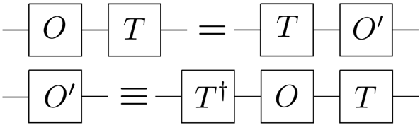
Figure 2 Operator pushing through an isometric tensor.
Figure 2 Operator pushing through an isometric tensor.CC-BY · From the PDF
Figure 3 If H A = H A 2 ⊗H A 1 , then we can move one of the factors to the output while preserving the isometric structure.
Figure 3 If H A = H A 2 ⊗H A 1 , then we can move one of the factors to the output while preserving the isometric structure.CC-BY · From the PDF
Figure 4 White dots represent physical legs on the boundary. Red dots represent logical input legs associated to each perfect tensor.
Figure 4 White dots represent physical legs on the boundary. Red dots represent logical input legs associated to each perfect tensor.CC-BY · From the PDF
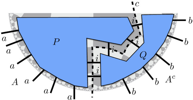
Figure 5 A cut through a holographic tensor network by a curve c bounded by ∂A . Boundary indices a and b are uncontracted in A and its complement A c respectively; tensors P and Q are contracted by summing over the index i which is cut by c .
Figure 5 A cut through a holographic tensor network by a curve c bounded by ∂A . Boundary indices a and b are uncontracted in A and its complement A c respectively; tensors P and Q are contracted by summing over the index i which is cut by c .CC-BY · From the PDF
Figure 6 A step in the greedy algorithm. The upper node has at least three legs contracted with the region P , which we have shaded red, so we include it into P .
Figure 6 A step in the greedy algorithm. The upper node has at least three legs contracted with the region P , which we have shaded red, so we include it into P .CC-BY · From the PDF
Figure 7 Three examples where the greedy algorithm fails to find the matching minimal geodesics from complementary regions. The first example involves disconnected regions in the holographic state. The second example involves a positive curvature obstruction at the center of the tiling which blocks the greedy geodesic from reaching the global minimal surface. The third example involves a connected region for the holographic code. In both the first and the third figure the greedy algorithm finds minimal geodesics from both sides but they do not match. In both cases, it is possible for the entropy to be slightly smaller than the length of the geodesic. This depends on tensors which were not absorbed by either of the greedy geodesics which we call the bipartite residual regions.
Figure 7 Three examples where the greedy algorithm fails to find the matching minimal geodesics from complementary regions. The first example involves disconnected regions in the holographic state. The second example involves a positive curvature obstruction at the center of the tiling which blocks the greedy geodesic from reaching the global minimal surface. The third example involves a connected region for the holographic code. In both the first and the third figure the greedy algorithm finds minimal geodesics from both sides but they do not match. In both cases, it is possible for the entropy to be slightly smaller than the length of the geodesic. This depends on tensors which were not absorbed by either of the greedy geodesics which we call the bipartite residual regions.CC-BY · From the PDF
Figure 8 The correspondence between local moves and distillation of EPR pairs. (a) Distillation of two EPR pairs. (b) The corresponding local moves. Before the first move, the tensor on the left has four legs crossed by the cut. Because the tensor is perfect, its remaining two legs are maximally entangled with a subsystem of these four. The first local unitary transformation acts on the four spins below the cut, transforming the basis to decouple the second and third spin, while the first and fourth spins remain contracted across the cut; in the corresponding local move, the cut advances upward past the tensor on the left. After the first move, the tensor on the right has five legs crossed by the cut. The second unitary transformation changes the basis of these five spins, decoupling the first four, while the fifth remains contracted across the cut; now the corresponding local move advances the cut upward past the tensor on the right. The product of the two local unitaries has distilled two EPR pairs which cross the cut, while decoupling six spins below the cut.
Figure 8 The correspondence between local moves and distillation of EPR pairs. (a) Distillation of two EPR pairs. (b) The corresponding local moves. Before the first move, the tensor on the left has four legs crossed by the cut. Because the tensor is perfect, its remaining two legs are maximally entangled with a subsystem of these four. The first local unitary transformation acts on the four spins below the cut, transforming the basis to decouple the second and third spin, while the first and fourth spins remain contracted across the cut; in the corresponding local move, the cut advances upward past the tensor on the left. After the first move, the tensor on the right has five legs crossed by the cut. The second unitary transformation changes the basis of these five spins, decoupling the first four, while the fifth remains contracted across the cut; now the corresponding local move advances the cut upward past the tensor on the right. The product of the two local unitaries has distilled two EPR pairs which cross the cut, while decoupling six spins below the cut.CC-BY · From the PDF
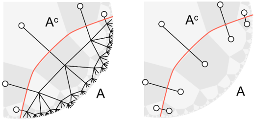
Figure 9 A geometric map of bipartite entanglement. White dots represent physical spins distilled by applying local unitary transformations to A and A c .
Figure 9 A geometric map of bipartite entanglement. White dots represent physical spins distilled by applying local unitary transformations to A and A c .CC-BY · From the PDF
Figure 10 The 'map of entanglement' and multipartite residual regions in a holographic state. For | A || C | ≫| B || D | it is possible for the residual region to pinch off so much that EPR pairs can be directly distilled between A and C . In other words, due to the discretization of the lattice, the causal wedges C [ A ] and C [ C ] may be adjacent in the bulk. In this case the residual region may be composed of two disconnected components, R B and R C which can contribute tripartite correlations. A similar analysis holds for | A || C | ≪| B || D | . For | A || C | ≈ | B || D | , a single connected residual region R contiguous to the four causal wedges is expected and may contribute four-party correlations.
Figure 10 The 'map of entanglement' and multipartite residual regions in a holographic state. For | A || C | ≫| B || D | it is possible for the residual region to pinch off so much that EPR pairs can be directly distilled between A and C . In other words, due to the discretization of the lattice, the causal wedges C [ A ] and C [ C ] may be adjacent in the bulk. In this case the residual region may be composed of two disconnected components, R B and R C which can contribute tripartite correlations. A similar analysis holds for | A || C | ≪| B || D | . For | A || C | ≈ | B || D | , a single connected residual region R contiguous to the four causal wedges is expected and may contribute four-party correlations.CC-BY · From the PDF
Figure 11 Bulk field reconstruction in the causal wedge. On the left is a spacetime diagram, showing the full spacetime extent of the causal wedge C [ A ] associated with a boundary subregion A that lies within a boundary time slice Σ. The point x lies within C [ A ] and thus any operator at x can be reconstructed on A . On the right is a bulk time slice containing x and Σ, which has a geometry similar to that of our tensor networks. The point x can simultaneously lie in distinct causal wedges, so φ ( x ) has multiple representations in the CFT.
Figure 11 Bulk field reconstruction in the causal wedge. On the left is a spacetime diagram, showing the full spacetime extent of the causal wedge C [ A ] associated with a boundary subregion A that lies within a boundary time slice Σ. The point x lies within C [ A ] and thus any operator at x can be reconstructed on A . On the right is a bulk time slice containing x and Σ, which has a geometry similar to that of our tensor networks. The point x can simultaneously lie in distinct causal wedges, so φ ( x ) has multiple representations in the CFT.CC-BY · From the PDF
Figure 12 Boundary reconstruction of bulk operators. The blue operator on the central bulk leg is pushed to an operator supported on a fairly large boundary region, while the green bulk operator further from the center is pushed to an operator supported on a smaller boundary region. Bulk legs for the other tensors are not shown.
Figure 12 Boundary reconstruction of bulk operators. The blue operator on the central bulk leg is pushed to an operator supported on a fairly large boundary region, while the green bulk operator further from the center is pushed to an operator supported on a smaller boundary region. Bulk legs for the other tensors are not shown.CC-BY · From the PDF
Figure 13 Disconnected reconstruction of a central operator beyond the causal wedge. Each of two separate connected boundary regions is too small for reconstruction of the central operator, yet the reconstruction is possible on the union of the two regions. In this example the greedy algorithm reaches the central tensor when applied to both connected components at once, but not when applied to either component by itself.
Figure 13 Disconnected reconstruction of a central operator beyond the causal wedge. Each of two separate connected boundary regions is too small for reconstruction of the central operator, yet the reconstruction is possible on the union of the two regions. In this example the greedy algorithm reaches the central tensor when applied to both connected components at once, but not when applied to either component by itself.CC-BY · From the PDF
Figure 14 The intersection of the entanglement wedge E [ A ] with a bulk time-slice, in the case where A has two connected components. Minimal geodesics in the bulk are solid lines. When A is smaller than A c , we have the situation on the left and the causal wedge agrees with the entanglement wedge. When A is bigger, however, the minimal geodesics switch and the entanglement wedge becomes larger. In particular the point in the center lies in the E [ A ] but not C [ A ].
Figure 14 The intersection of the entanglement wedge E [ A ] with a bulk time-slice, in the case where A has two connected components. Minimal geodesics in the bulk are solid lines. When A is smaller than A c , we have the situation on the left and the causal wedge agrees with the entanglement wedge. When A is bigger, however, the minimal geodesics switch and the entanglement wedge becomes larger. In particular the point in the center lies in the E [ A ] but not C [ A ].CC-BY · From the PDF
Figure 15 (a) When a boundary region A is partitioned into many connected components it may have a very shallow causal wedge C [ A ] if each connected component is small. (b) In contrast, if A comprises a sufficiently large fraction of the boundary, its entanglement wedge E [ A ] will extend deep into the bulk.
Figure 15 (a) When a boundary region A is partitioned into many connected components it may have a very shallow causal wedge C [ A ] if each connected component is small. (b) In contrast, if A comprises a sufficiently large fraction of the boundary, its entanglement wedge E [ A ] will extend deep into the bulk.CC-BY · From the PDF
Figure 16 Dangerous small erasures for the triangle (a) and pentagon codes (b). In the triangle code erasing two boundary spins, boxed in blue, can prevent reconstruction of the central tensor. In the pentagon code erasing four spins can prevent the reconstruction.
Figure 16 Dangerous small erasures for the triangle (a) and pentagon codes (b). In the triangle code erasing two boundary spins, boxed in blue, can prevent reconstruction of the central tensor. In the pentagon code erasing four spins can prevent the reconstruction.CC-BY · From the PDF
Figure 17 Tensor networks for holographic pentagon/hexagon codes with erasure thresholds, where neighboring polygons share contracted indices. In the network shown on the left, pentagons and hexagons alternate on the lattice; each pentagon carries one dangling bulk index, and hexagons carry no bulk degrees of freedom. The logical qubit residing on the central pentagon is well protected against erasure if the erasure probability on the boundary is below the threshold value p c . In the network on the right, there is just a single bulk qubit located at the center; the rest of the network is similar to the holographic state constructed from hexagons only.
Figure 17 Tensor networks for holographic pentagon/hexagon codes with erasure thresholds, where neighboring polygons share contracted indices. In the network shown on the left, pentagons and hexagons alternate on the lattice; each pentagon carries one dangling bulk index, and hexagons carry no bulk degrees of freedom. The logical qubit residing on the central pentagon is well protected against erasure if the erasure probability on the boundary is below the threshold value p c . In the network on the right, there is just a single bulk qubit located at the center; the rest of the network is similar to the holographic state constructed from hexagons only.CC-BY · From the PDF
Figure 18 A black hole in a holographic code, and the corresponding wormhole geometry.
Figure 18 A black hole in a holographic code, and the corresponding wormhole geometry.CC-BY · From the PDF
Figure 19 Here we illustrate how to construct a unitary circuit interpretation of a holographic state which witnesses the RT entanglement for a simply connected boundary region. (a) The following steps for the construction are illustrated: i) Label the node located at one end of the boundary as 0. ii) Label all other nodes according to the distance from this node. iii) Direct all tensor indices such that the larger label lies to the right. (b) In the example, the circuit interpretation for the network has depth 12. For this reason we provide a full sequential presentation of the circuit interpretation along one side of the geodesic, condensing the remaining 7 gates into U A c . Note that there are outputs that are produced directly by U A , without going through U A c as well as inputs that are fed directly to U A c without going through U A .
Figure 19 Here we illustrate how to construct a unitary circuit interpretation of a holographic state which witnesses the RT entanglement for a simply connected boundary region. (a) The following steps for the construction are illustrated: i) Label the node located at one end of the boundary as 0. ii) Label all other nodes according to the distance from this node. iii) Direct all tensor indices such that the larger label lies to the right. (b) In the example, the circuit interpretation for the network has depth 12. For this reason we provide a full sequential presentation of the circuit interpretation along one side of the geodesic, condensing the remaining 7 gates into U A c . Note that there are outputs that are produced directly by U A , without going through U A c as well as inputs that are fed directly to U A c without going through U A .CC-BY · From the PDF
Figure 21 The best-case reconstruction of the center; we need to use only three 'branches' of the tree, and in the outer branches we can choose to push 'inwards' every time.
Figure 21 The best-case reconstruction of the center; we need to use only three 'branches' of the tree, and in the outer branches we can choose to push 'inwards' every time.CC-BY · From the PDF
Figure 22 The worst-case reconstruction of the center; we are just barely not able to use the second branch, so we need to use the third, fourth, and fifth.
Figure 22 The worst-case reconstruction of the center; we are just barely not able to use the second branch, so we need to use the third, fourth, and fifth.CC-BY · From the PDF
Figure 23 Locations of the 'bad' points from figure 16b. If the worst-case region were just a little smaller on the right it wouldn't contain any of them so, it wouldn't be able to reconstruct the center.
Figure 23 Locations of the 'bad' points from figure 16b. If the worst-case region were just a little smaller on the right it wouldn't contain any of them so, it wouldn't be able to reconstruct the center.CC-BY · From the PDF
Image 23
CC-BY · From the PDF
| {z } ≥ 1 erasure. | {z } ≥ Figure 25 . We illustrate the prerequisite for two erasures to be propagated one layer higher. The most fragile case corresponds to one of the sites having only four descendants since at least one of them needs to have five. Irrespective of the availability of a shared descendant there is a minimum number of erasures that need to occur in order to propagate two contiguous erasures.
| {z } ≥ 1 erasure. | {z } ≥ Figure 25 . We illustrate the prerequisite for two erasures to be propagated one layer higher. The most fragile case corresponds to one of the sites having only four descendants since at least one of them needs to have five. Irrespective of the availability of a shared descendant there is a minimum number of erasures that need to occur in order to propagate two contiguous erasures.CC-BY · From the PDF
Figure 26 Here we present Monte Carlo simulation for the probability of the central tensor being incorporated by the greedy algorithm applied to a holographic code. The greedy algorithm is applied to a region A constructed by randomly taking each boundary physical index to belong to A with probability p . We plot the central tensor containment probability in the greedy wedge according to the lattice radius (i.e. the distance from the central tensor at which the a priory infinite network is truncated). (a) We consider the holographic pentagon code of figure 4b. Numerical results remains consistent with the existence of five possible weight 4 representations of the string-like logical operators acting on the central qubit. (b) We focus on the pentagon/hexagon code of figure 17a which has an erasure threshold in terms of the recoverabilty. We observe some oscillatory behavior due to the fact that tensor 'layers' added alternate between pentagons and hexagons. (c) We present numerical data for the greedy algorithm applied to the 1 qubit hexagon code of figure 17b which corresponds to a tensor network identical to the holographic hexagon state except for having a single pentagon at its center.
Figure 26 Here we present Monte Carlo simulation for the probability of the central tensor being incorporated by the greedy algorithm applied to a holographic code. The greedy algorithm is applied to a region A constructed by randomly taking each boundary physical index to belong to A with probability p . We plot the central tensor containment probability in the greedy wedge according to the lattice radius (i.e. the distance from the central tensor at which the a priory infinite network is truncated). (a) We consider the holographic pentagon code of figure 4b. Numerical results remains consistent with the existence of five possible weight 4 representations of the string-like logical operators acting on the central qubit. (b) We focus on the pentagon/hexagon code of figure 17a which has an erasure threshold in terms of the recoverabilty. We observe some oscillatory behavior due to the fact that tensor 'layers' added alternate between pentagons and hexagons. (c) We present numerical data for the greedy algorithm applied to the 1 qubit hexagon code of figure 17b which corresponds to a tensor network identical to the holographic hexagon state except for having a single pentagon at its center.CC-BY · From the PDF
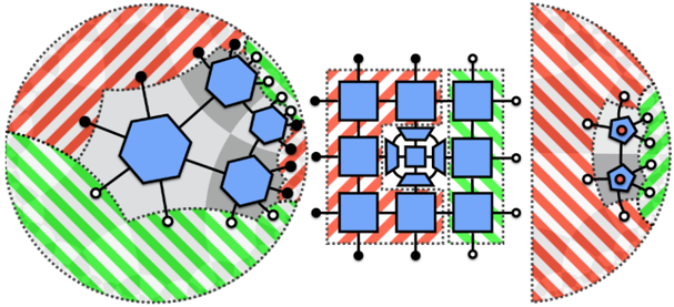
Figure 27 In (a) we represent a bipartite network composed of tensors with a symmetry H and H ∗ . We alternate applying H (solid squares) and H ∗ (hollow squares) to all legs of tensors in the bipartite tensor network. In (b) we represent the same tensor network where a portion A of the boundary was marked with hollow dots and its complement A c was marked with full dots. The regions A and A c have been chosen such that the greedy algorithm does not progress on either. The greedy algorithm will recover the full network when initiated from the full boundary showing that the network indeed corresponds to a holographic code.
Figure 27 In (a) we represent a bipartite network composed of tensors with a symmetry H and H ∗ . We alternate applying H (solid squares) and H ∗ (hollow squares) to all legs of tensors in the bipartite tensor network. In (b) we represent the same tensor network where a portion A of the boundary was marked with hollow dots and its complement A c was marked with full dots. The regions A and A c have been chosen such that the greedy algorithm does not progress on either. The greedy algorithm will recover the full network when initiated from the full boundary showing that the network indeed corresponds to a holographic code.CC-BY · From the PDF

Verification

Claims the paper makes

The claims and statistics of this paper haven’t been checked yet.

Free: it reads the open-access text and checks the first 5 claims that cite a source we can check. Create a free account to check every claim.

A few free checks a day · papers already verified open instantly · results are public

Claims other papers make about this one

Each is checked against this paper’s own text: does it say what the citing paper says it does?

2 more claims about this paper

Create a free account to see every claim other papers make about this one.

See all claims — free account

Self-check

Percentages, sums and reported differences re-computed from the paper’s own numbers.

The self-check needs the paper’s full text.

Citations

Cites

Show all 67 references

Research works printed but not linked: 5

  1. 45. E. Mintun, J. Polchinski and V. Rosenhaus, Bulk-boundary duality, gauge invariance and quantum error correction, arXiv:1501.06577 [INSPIRE]. · arXiv
  2. 53. L. Susskind, Computational complexity and black hole horizons, arXiv:1403.5695 [INSPIRE]. · arXiv
  3. 59. J. Adler, Bootstrap percolation, Phys. A 171 (1991) 453.
  4. 61. M.A. Nielsen and I.L. Chuang, Quantum computation and quantum information, Cambridge University Press, Cambridge U.K. (2000).
  5. 63. M.B. S ¸ahinoglu et al., Characterizing topological order with matrix product operators, arXiv:1409.2150. · arXiv

Cited by

See all 1,006

Metadata

Authors
Pastawski, F., Yoshida, B., Harlow, D., & Preskill, J.
Affiliations
  • California Institute of Technology (US)
  • Princeton University (US)
Corresponding author
Pastawski, Fernando
Venue
Journal of High Energy Physics
Published
2015-06
Volume
2015
Issue
6
ISSN
1029-8479 (ISSN-L)
OpenAlex
W1934222401
Cited by
958
References
46
Citations by year
2026: 64 · 2025: 95 · 2024: 91 · 2023: 82 · 2022: 99 · 2021: 95 · 2020: 122 · 2019: 103 · 2018: 76 · 2017: 77 · 2016: 35 · 2015: 18
FWCI
34.52
Type
journal article
Language
en
Open access
Licence
cc-by
Locations
  • Journal of High Energy Physics (publishedVersion, cc-by)
  • arXiv (Cornell University) (submittedVersion)
  • CaltechAUTHORS (California Institute of Technology) (submittedVersion, cc-by)
  • arXiv (Cornell University)
Funders
  • National Science Foundation (1125565, 0803371)
  • Gordon and Betty Moore Foundation (PHY-1125565, PHY-0803371)
  • Institute for Quantum Information and Matter, California Institute of Technology (PHY-1125565)
Topics
  • Physical Sciences › Physics and Astronomy › Nuclear and High Energy Physics › Black Holes and Theoretical Physics
  • Physical Sciences › Physics and Astronomy › Atomic and Molecular Physics, and Optics › Quantum many-body systems
  • Physical Sciences › Physics and Astronomy › Nuclear and High Energy Physics › Noncommutative and Quantum Gravity Theories
Keywords
AdS/CFT correspondence, bulk-boundary correspondence, tensor networks, Ryu-Takayanagi formula, holographic entanglement

About these checks

Registry, retraction, Cites and statistics results are computed, not judged, with one exception: a printed reference that no index lists is read once by a model before it counts as a citation error. Claims are extracted by a model and kept only when their quote appears verbatim in the text; each cited source is then checked, with a model’s help, for whether it says what the claim relies on. Those verdicts can be wrong — read the claim’s quote and the cited source before relying on one.

Statistics and arithmetic are recomputed, not judged.

Confidence bands are shown only for fields calibrated on our annotated test set. None is calibrated yet, so no band is shown.

What counts as a claim ›How we measure confidence ›How we check this ›

Are you an author, or do you see a problem with this page? Request a review

Data sources

Bibliographic data: Semantic Scholar, OpenAlex, Crossref.

Contains information from the Semantic Scholar Academic Graph Datasets, made available under the ODC Attribution License (ODC-BY 1.0).

Semantic Scholar’s data is described in: Kinney, R., et al. (2023). The Semantic Scholar Open Data Platform. arXiv:2301.10140.