

The DOI matches its Crossref record; 72 of the 72 references it cites were found in a registry or an index.
Numerical Solution of the Parametric Diffusion Equation by Deep Neural Networks
Abstract
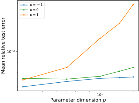
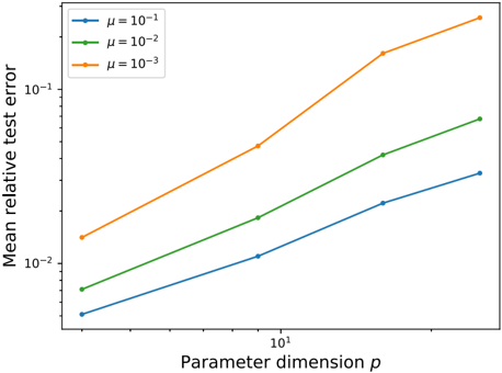
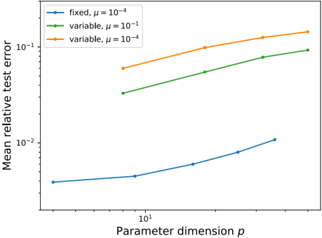
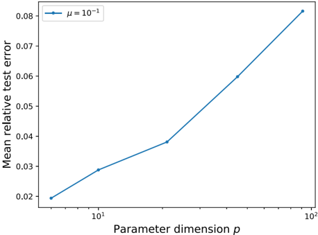
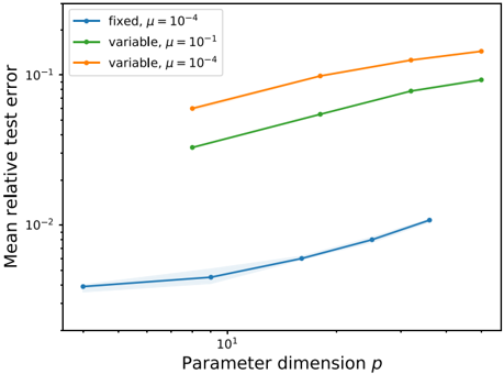
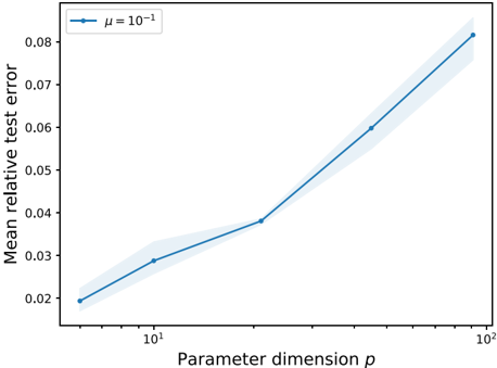
We perform a comprehensive numerical study of the effect of approximation-theoretical results for neural networks on practical learning problems in the context of numerical analysis. As the underlying model, we study the machine-learning-based solution of parametric partial differential equations. Here, approximation theory for fully-connected neural networks predicts that the performance of the model should depend only very mildly on the dimension of the parameter space and is determined by the intrinsic dimension of the solution manifold of the parametric partial differential equation. We use various methods to establish comparability between test-cases by minimizing the effect of the choice of test-cases on the optimization and sampling aspects of the learning problem. We find strong support for the hypothesis that approximation-theoretical effects heavily influence the practical behavior of learning problems in numerical analysis. Turning to practically more successful and modern architectures, at the end of this study we derive improved error bounds by focusing on convolutional neural networks.
Overview
The claims and statistics of this paper haven’t been checked yet.
Run the check — free, no account needed. It reads the open-access text and checks the sources it cites.
Integrity signals
Registry
Cites
Statistics
Figures
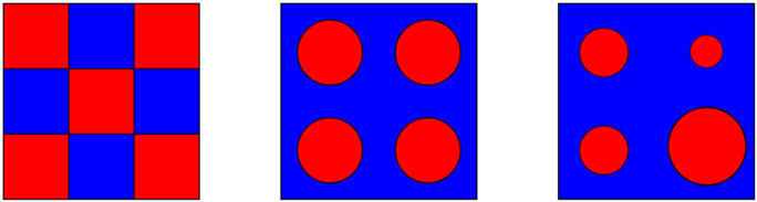
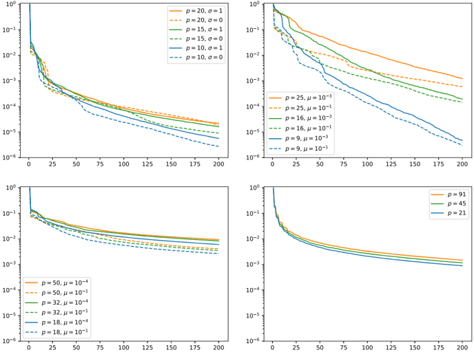
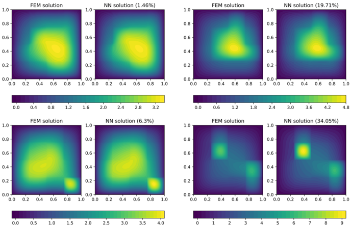
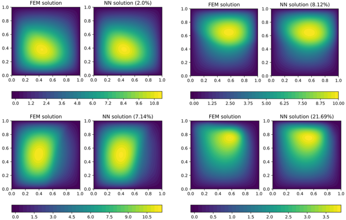
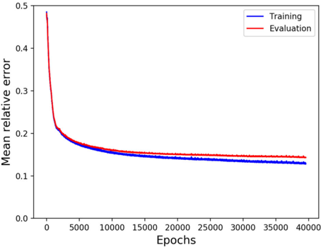
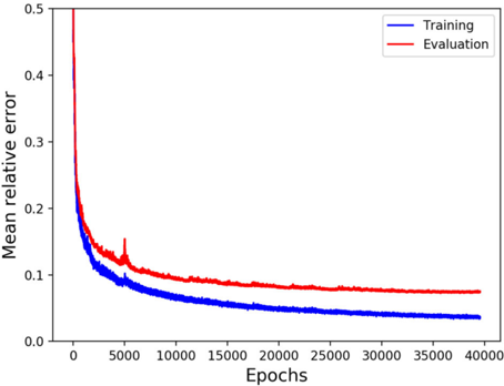
Verification
Claims the paper makes
The claims and statistics of this paper haven’t been checked yet.
Run the check — free, no account needed. It reads the open-access text and checks the sources it cites.
Claims other papers make about this one
Each is checked against this paper’s own text: does it say what the citing paper says it does?
In the citing paper
“Incorporating the current 2σ bound on the tensor/scalar ratio r [75, 76] requires roughly H/M P < 10 -7 .”
From Hyperbolic compactification of M-theory and de Sitter quantum gravity (2022) · cites this paper as [76]
Self-check
Percentages, sums and reported differences re-computed from the paper’s own numbers.
The self-check needs the paper’s full text.
Citations
Cites
Adam: A Method for Stochastic Optimization
Kingma, D. P., & Ba, J. (2014) · arXiv · doi:10.48550/arxiv.1412.6980 · Cited by 98,946
Gradient-based learning applied to document recognition
Lecun, Y., Bottou, L., Bengio, Y., & Haffner, P. (1998) · Proceedings of the IEEE · doi:10.1109/5.726791 · Cited by 58,805
Universal approximation bounds for superpositions of a sigmoidal function
Barron, A. R. (1993) · IEEE Transactions on Information Theory · doi:10.1109/18.256500 · Cited by 2,804
DeepXDE: A Deep Learning Library for Solving Differential Equations
Lu, L., Meng, X., Mao, Z., & Karniadakis, G. E. (2021) · SIAM Review · doi:10.1137/19m1274067 · Cited by 2,512
Artificial neural networks for solving ordinary and partial differential equations
Lagaris, I. E., Likas, A., & Fotiadis, D. I. (1998) · IEEE Transactions on Neural Networks · doi:10.1109/72.712178 · Cited by 2,412
SchNet – A deep learning architecture for molecules and materials
Schütt, K. T., Sauceda, H. E., Kindermans, P.-J., Tkatchenko, A., & Müller, K.-R. (2018) · The Journal of Chemical Physics · doi:10.1063/1.5019779 · Cited by 2,217
DGM: A deep learning algorithm for solving partial differential equations
Sirignano, J., & Spiliopoulos, K. (2018) · Journal of Computational Physics · doi:10.1016/j.jcp.2018.08.029 · Cited by 2,208
Samaniego, E., Anitescu, C., Goswami, S., Nguyen-Thanh, V. M., Guo, H., Hamdia, K., Zhuang, X., & Rabczuk, T. (2020) · Computer Methods in Applied Mechanics and Engineering · doi:10.1016/j.cma.2019.112790 · Cited by 2,104
The FEniCS Project Version 1.5
Alnæs, M. S., Blechta, J., Hake, J. E., Johansson, A., Kehlet, B., Logg, A., Richardson, C., Ring, J., Rognes, M. E., & Wells, G. N. (2015) · Department of Earth Sciences EPrints Repository · doi:10.11588/ans.2015.100.20553 · Cited by 1,877
Solving high-dimensional partial differential equations using deep learning
Han, J., Jentzen, A., & E, W. (2018) · Proceedings of the National Academy of Sciences · doi:10.1073/pnas.1718942115 · Cited by 1,722
On the mathematical foundations of learning
Cucker, F., & Smale, S. (2001) · Bulletin of the American Mathematical Society · doi:10.1090/s0273-0979-01-00923-5 · Cited by 1,545
Mathematical Statistics With Applications
Meek, G. E. (1987) · Technometrics · doi:10.1080/00401706.1987.10488256 · Cited by 1,425
The Deep Ritz Method: A Deep Learning-Based Numerical Algorithm for Solving Variational Problems
E, W., & Yu, B. (2018) · Communications in Mathematics and Statistics · doi:10.1007/s40304-018-0127-z · Cited by 1,418
Hidden physics models: Machine learning of nonlinear partial differential equations
Raissi, M., & Karniadakis, G. E. (2018) · Journal of Computational Physics · doi:10.1016/j.jcp.2017.11.039 · Cited by 1,349
Rozza, G., Huynh, D. B. P., & Patera, A. T. (2008) · Archives of Computational Methods in Engineering · doi:10.1007/s11831-008-9019-9 · Cited by 1,108
Error bounds for approximations with deep ReLU networks
Yarotsky, D. (2017) · Neural Networks · doi:10.1016/j.neunet.2017.07.002 · Cited by 1,085
Certified Reduced Basis Methods for Parametrized Partial Differential Equations
Hesthaven, J. S., Rozza, G., & Stamm, B. (2016) · SpringerBriefs in Mathematics · doi:10.1007/978-3-319-22470-1 · Cited by 1,039
On the theory of dynamic programming
Bellman, R. (1952) · Proceedings of the National Academy of Sciences · doi:10.1073/pnas.38.8.716 · Cited by 998
Artificial Neural Networks for Solving Ordinary and Partial Differential Equations
Lagaris, I. E., Likas, A., & Fotiadis, D. I. (1998) · Cited by 944
Raissi, M., Perdikaris, P. G., & Karniadakis, G. E. (2017) · arXiv (Cornell University) · doi:10.48550/arxiv.1711.10561 · Cited by 925
E, W., Han, J., & Jentzen, A. (2017) · Communications in Mathematics and Statistics · doi:10.1007/s40304-017-0117-6 · Cited by 822
Model reduction of dynamical systems on nonlinear manifolds using deep convolutional autoencoders
Lee, K., & Carlberg, K. T. (2020) · Journal of Computational Physics · doi:10.1016/j.jcp.2019.108973 · Cited by 752
Prediction Errors of Molecular Machine Learning Models Lower than Hybrid DFT Error
Faber, F. A., Hutchison, L., Huang, B., Gilmer, J., Schoenholz, S. S., Dahl, G. E., Vinyals, O., Kearnes, S., Riley, P. F., & von Lilienfeld, O. A. (2017) · Journal of Chemical Theory and Computation · doi:10.1021/acs.jctc.7b00577 · Cited by 651
Non-intrusive reduced order modeling of nonlinear problems using neural networks
Hesthaven, J. S., & Ubbiali, S. (2018) · Journal of Computational Physics · doi:10.1016/j.jcp.2018.02.037 · Cited by 616
Reduced Basis Methods for Partial Differential Equations
Quarteroni, A. M., Manzoni, A., & Negri, F. (2015) · Unitext · doi:10.1007/978-3-319-15431-2 · Cited by 562
Why and when can deep-but not shallow-networks avoid the curse of dimensionality: A review
Poggio, T., Mhaskar, H., Rosasco, L., Miranda, B., & Liao, Q. (2017) · International Journal of Automation and Computing · doi:10.1007/s11633-017-1054-2 · Cited by 559
An Introduction to Computational Stochastic PDEs
Lord, G. J., Powell, C. E., & Shardlow, T. (2014) · Cambridge University Press eBooks · doi:10.1017/cbo9781139017329 · Cited by 537
Deep-neural-network solution of the electronic Schrödinger equation
Hermann, J., Schätzle, Z., & Noé, F. (2020) · Nature Chemistry · doi:10.1038/s41557-020-0544-y · Cited by 503
Learning Theory: An Approximation Theory Viewpoint
Felipe Cucker, B., & Zhou, D. X. (2007) · Cited by 478
Tripathy, R. K., & Bilionis, I. (2018) · Journal of Computational Physics · doi:10.1016/j.jcp.2018.08.036 · Cited by 464
Felipe Cucker, B., & Zhou, D. X. (2007) · Cambridge University Press eBooks · doi:10.1017/cbo9780511618796 · Cited by 433
Optimal approximation of piecewise smooth functions using deep ReLU neural networks
Petersen, P., & Voigtlaender, F. (2018) · Neural Networks · doi:10.1016/j.neunet.2018.08.019 · Cited by 432
Self-citationNeural Networks for Optimal Approximation of Smooth and Analytic Functions
Mhaskar, H. N. (1996) · Neural Computation · doi:10.1162/neco.1996.8.1.164 · Cited by 321
Beck, C., E, W., & Jentzen, A. (2019) · Journal of Nonlinear Science · doi:10.1007/s00332-018-9525-3 · Cited by 308
Hierarchical modeling of molecular energies using a deep neural network
Lubbers, N., Smith, J. S., & Barros, K. (2018) · The Journal of Chemical Physics · doi:10.1063/1.5011181 · Cited by 306
Theory of deep convolutional neural networks: Downsampling
Zhou, D.-X. (2020) · Neural Networks · doi:10.1016/j.neunet.2020.01.018 · Cited by 263
Approximation of high-dimensional parametric PDEs
Cohen, A. K., & DeVore, R. (2015) · Acta Numerica · doi:10.1017/s0962492915000033 · Cited by 259
Deep Network Approximation for Smooth Functions
Lu, J., Shen, Z., Yang, H., & Zhang, S. (2021) · SIAM Journal on Mathematical Analysis · doi:10.1137/20m134695x · Cited by 246
Optimal Approximation with Sparsely Connected Deep Neural Networks
Bölcskei, H., Grohs, P., Gitta Kutyniok, B., & Petersen, P. (2019) · SIAM Journal on Mathematics of Data Science · doi:10.1137/18m118709x · Cited by 245
Self-citationProvable approximation properties for deep neural networks
Shaham, U., Cloninger, A., & Coifman, R. R. (2016) · Applied and Computational Harmonic Analysis · doi:10.1016/j.acha.2016.04.003 · Cited by 206
A Theoretical Analysis of Deep Neural Networks and Parametric PDEs
Gitta Kutyniok, B., Petersen, P., Raslan, M., & Schneider, R. (2021) · Constructive Approximation · doi:10.1007/s00365-021-09551-4 · Cited by 194
Self-citationSchwab, C., & Zech, J. (2018) · Analysis and Applications · doi:10.1142/s0219530518500203 · Cited by 192
An artificial neural network framework for reduced order modeling of transient flows
San, O., Maulik, R., & Ahmed, M. (2019) · Communications in Nonlinear Science and Numerical Simulation · doi:10.1016/j.cnsns.2019.04.025 · Cited by 170
Grohs, P., Hornung, F., Jentzen, A., & von Wurstemberger, P. (2023) · Memoirs of the American Mathematical Society · doi:10.1090/memo/1410 · Cited by 165
Data-driven discovery of PDEs in complex datasets
Berg, J., & Nyström, K. (2019) · Journal of Computational Physics · doi:10.1016/j.jcp.2019.01.036 · Cited by 153
The Gap between Theory and Practice in Function Approximation with Deep Neural Networks
Adcock, B., & Dexter, N. (2021) · SIAM Journal on Mathematics of Data Science · doi:10.1137/20m131309x · Cited by 152
The Random Feature Model for Input-Output Maps between Banach Spaces
Nelsen, N. H., & Stuart, A. M. (2021) · SIAM Journal on Scientific Computing · doi:10.1137/20m133957x · Cited by 151
Optimal approximation of continuous functions by very deep ReLU networksPreprint
Yarotsky, D. (2018) · arXiv (Cornell University) · doi:10.48550/arxiv.1802.03620 · Cited by 136
Machine learning for fast and reliable solution of time-dependent differential equations
Regazzoni, F., Dede’, L., & Quarteroni, A. M. (2019) · Journal of Computational Physics · doi:10.1016/j.jcp.2019.07.050 · Cited by 129
Deep ReLU networks and high-order finite element methods
Opschoor, J. A. A., Petersen, P., & Schwab, C. (2019) · Analysis and Applications · doi:10.1142/s0219530519410136 · Cited by 110
Self-citationDNN Expression Rate Analysis of High-Dimensional PDEs: Application to Option Pricing
Elbrächter, D., Grohs, P., Jentzen, A., & Schwab, C. (2021) · Constructive Approximation · doi:10.1007/s00365-021-09541-6 · Cited by 101
Hutzenthaler, M., Jentzen, A., Kruse, T., & Nguyen, T. A. (2020) · Partial Differential Equations and Applications · doi:10.1007/s42985-019-0006-9 · Cited by 83
Solving stochastic differential equations and Kolmogorov equations by means of deep learningPreprint
Beck, C., Becker, S. B. S., Grohs, P., Jaafari, N., & Jentzen, A. (2018) · arXiv (Cornell University) · Cited by 82
Equivalence of approximation by convolutional neural networks and fully-connected networks
Petersen, P., & Voigtlaender, F. (2019) · Proceedings of the American Mathematical Society · doi:10.1090/proc/14789 · Cited by 77
Self-citationPhysics-informed deep generative modelsPreprint
Yang, Y., & Perdikaris, P. G. (2018) · arXiv (Cornell University) · doi:10.48550/arxiv.1812.03511 · Cited by 76
Data driven approximation of parametrized PDEs by reduced basis and neural networks
Santo, N. D., Simone Deparis, A., & Pegolotti, L. (2020) · Journal of Computational Physics · doi:10.1016/j.jcp.2020.109550 · Cited by 69
Approximation of infinitely differentiable multivariate functions is intractable
Novak, E., & Woźniakowski, H. (2008) · Journal of Complexity · doi:10.1016/j.jco.2008.11.002 · Cited by 65
Kolmogorov widths and low-rank approximations of parametric elliptic PDEs
Bachmayr, M., & Cohen, A. K. (2016) · Mathematics of Computation · doi:10.1090/mcom/3132 · Cited by 64
Han, J., Nica, M., & Stinchcombe, A. R. (2020) · Journal of Computational Physics · doi:10.1016/j.jcp.2020.109672 · Cited by 62
Compressive sensing Petrov-Galerkin approximation of high-dimensional parametric operator equations
Rauhut, H., & Schwab, C. (2015) · Mathematics of Computation · doi:10.1090/mcom/3113 · Cited by 52
Brevis, I., Muga, I., & Zee, K. G. V. D. (2020) · Computers & Mathematics with Applications · doi:10.1016/j.camwa.2020.08.012 · Cited by 43
Efficient approximation of solutions of parametric linear transport equations by ReLU DNNs
Laakmann, F., & Petersen, P. (2021) · Advances in Computational Mathematics · doi:10.1007/s10444-020-09834-7 · Cited by 42
Self-citationHan, J., Jentzen, A., & Weinan, E. (2017) · Cited by 40
ANALYTIC REGULARITY AND POLYNOMIAL APPROXIMATION OF STOCHASTIC, PARAMETRIC ELLIPTIC MULTISCALE PDEs
Hòang, V. H., & Schwab, C. (2012) · Analysis and Applications · doi:10.1142/s0219530513500012 · Cited by 38
A multi-level procedure for enhancing accuracy of machine learning algorithms
Lye, K. O., Mishra, S., & Molinaro, R. (2020) · European Journal of Applied Mathematics · doi:10.1017/s0956792520000224 · Cited by 36
Reduced Basis Methods: Success, Limitations and Future ChallengesPreprint
Ohlberger, M., & Rave, S. (2015) · arXiv (Cornell University) · doi:10.48550/arxiv.1511.02021 · Cited by 32
Parametric PDEs: sparse or low-rank approximations?
Bachmayr, M., Cohen, A. K., & Dahmen, W. (2017) · IMA Journal of Numerical Analysis · doi:10.1093/imanum/drx052 · Cited by 32
Deep neural network expression of posterior expectations in Bayesian PDE inversion *
Herrmann, L., Schwab, C., & Zech, J. (2020) · Inverse Problems · doi:10.1088/1361-6420/abaf64 · Cited by 30
Eigel, M., Schneider, R., Trunschke, P., & Wolf, S. (2019) · Advances in Computational Mathematics · doi:10.1007/s10444-019-09723-8 · Cited by 24
Self-citationGrowing axons: greedy learning of neural networks with application to function approximation
Fokina, D., & Oseledets, I. V. (2023) · Russian Journal of Numerical Analysis and Mathematical Modelling · doi:10.1515/rnam-2023-0001 · Cited by 13
Deep ReLU Neural Network Expression Rates for Data-to-QoI Maps in Bayesian PDE Inversion
Herrmann, L., Schwab, C., & Zech, J. (2020) · SAM Research Report · Cited by 10
A mixed ℓ1 regularization approach for sparse simultaneous approximation of parameterized PDEs
Dexter, N., Tran, H., & Webster, C. (2019) · ESAIM Mathematical Modelling and Numerical Analysis · doi:10.1051/m2an/2019048 · Cited by 8
Research works printed but not linked: 8
- Adcock, B., Brugiapaglia, S., Dexter, N., Moraga, S.: Deep neural networks are effective at learning high-dimensional Hilbert-valued functions from limited data. arXiv preprint arXiv:2012.06081 (2020) · arXiv
- Berner, J., Grohs, P., Jentzen, A.: Analysis of the generalization error: empirical risk minimization over deep artificial neural networks overcomes the curse of dimensionality in the numerical approximation of Black-Scholes partial differential equations. arXiv preprint arXiv:1809.03062 (2018) · arXiv
- Bhattacharya, K., Hosseini, B., Kovachki, N.B., Stuart, A.M.: Model reduction and neural networks for parametric PDEs. arXiv preprintarXiv:2005.03180 (2020)
- Brevis, I., Muga, I., van der Zee, K.G.: Data-driven finite elements methods: machine learning acceleration of goal-oriented computations. arXiv preprint arXiv:2003.04485 (2020) · arXiv
- Jentzen, A., Salimova, D., Welti, T.: A proof that deep artificial neural networks overcome the curse of dimensionality in the numerical approximation of Kolmogorov partial differential equations with constant diffusion and nonlinear drift coefficients. arXiv preprintarXiv:1809.07321 (2018)
- Khoo, Y., Lu, J., Ying, L.: Solving parametric PDE problems with artificial neural networks. arXiv preprint arXiv:1707.03351 (2017) · arXiv
- Marcati, C., Opschoor, J.A., Petersen, P.C., Schwab, C.: Exponential relu neural network approximation rates for point and edge singularities. arXiv preprint arXiv:2010.12217 (2020) · arXiv
- Raissi, M., Perdikaris, P., Karniadakis, G.E.: Physics informed deep learning (part ii): data-driven discovery of nonlinear partial differential equations. arxiv. arXiv preprint arXiv:1711.10561, (2017) · arXiv
Cited by
Hyperbolic compactification of M-theory and de Sitter quantum gravity
De Luca, G. B., Silverstein, E., & Torroba, G. (2022) · SciPost Physics · doi:10.21468/scipostphys.12.3.083 · Cited by 39
Metadata
- Authors
- Geist, M., Petersen, P., Raslan, M., Schneider, R., & Kutyniok, G.
- Venue
- Journal of Scientific Computing
- Published
- 2021-06-05
- Volume
- 88
- Issue
- 1
- ISSN
- 0885-7474
- 1573-7691
- Cited by
- 57
- References
- 72
- Language
- en
- Licence
- creativecommons.org/licenses/by/4.0 (tdm)
- creativecommons.org/licenses/by/4.0 (vor)
- Funders
- University of Vienna
About these checks
Registry, retraction, Cites and statistics results are computed, not judged, with one exception: a printed reference that no index lists is read once by a model before it counts as a citation error. Claims are extracted by a model and kept only when their quote appears verbatim in the text; each cited source is then checked, with a model’s help, for whether it says what the claim relies on. Those verdicts can be wrong — read the claim’s quote and the cited source before relying on one.
Statistics and arithmetic are recomputed, not judged.
Confidence bands are shown only for fields calibrated on our annotated test set. None is calibrated yet, so no band is shown.
What counts as a claim ›How we measure confidence ›How we check this ›
Are you an author, or do you see a problem with this page? Request a review
Data sources
Bibliographic data: Semantic Scholar, OpenAlex, Crossref.
Contains information from the Semantic Scholar Academic Graph Datasets, made available under the ODC Attribution License (ODC-BY 1.0).
Semantic Scholar’s data is described in: Kinney, R., et al. (2023). The Semantic Scholar Open Data Platform. arXiv:2301.10140.
