

The DOI matches its Crossref record; 59 of the 59 references it cites were found in a registry or an index.
Cell-TIMP: Cellular Trajectory Inference Based on Morphological Parameters
Open accessPublished version of a preprint
Abstract
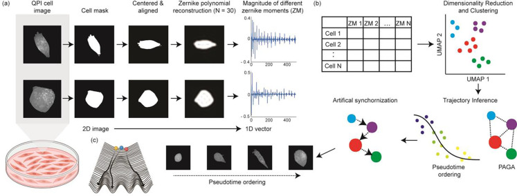
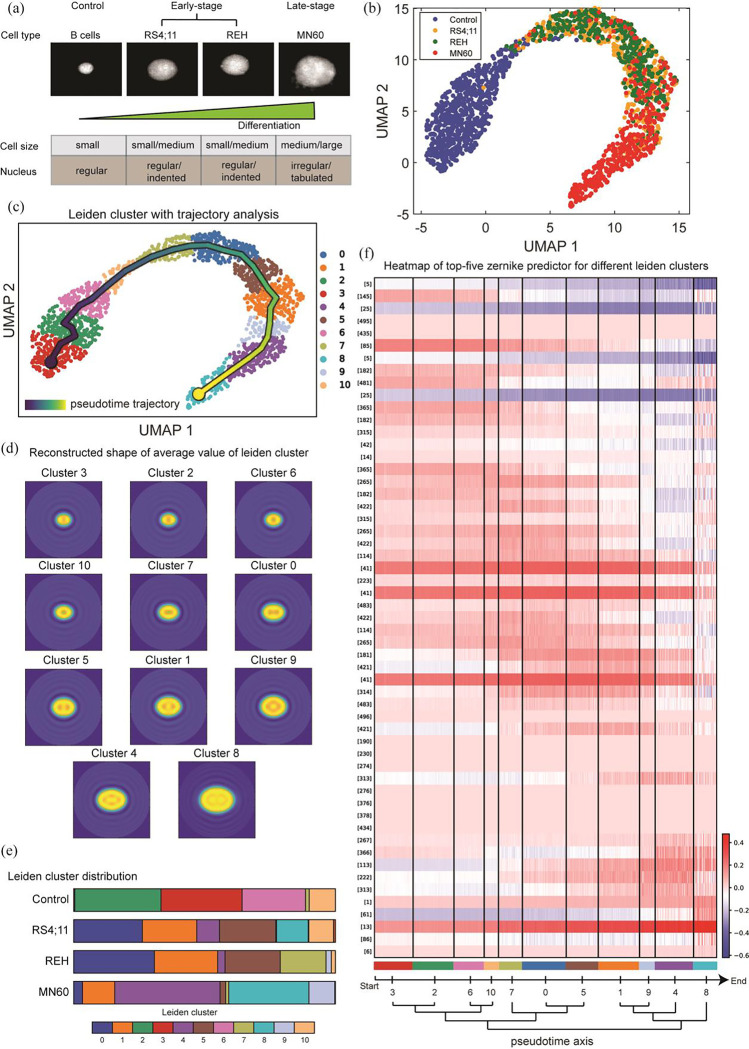
Cellular morphology, shaped by various genetic and environmental influences, is pivotal to studying experimental cell biology, necessitating precise measurement and analysis techniques. Traditional approaches, which rely on geometric metrics derived from stained images, encounter obstacles stemming from both the imaging and analytical domains. Staining processes can disrupt the cell's natural state and diminish accuracy due to photobleaching, while conventional analysis techniques, which categorize cells based on shape to discern pathophysiological conditions, often fail to capture the continuous and asynchronous nature of biological processes such as cell differentiation, immune responses, and cancer progression. In this work, we propose the use of quantitative phase imaging for morphological assessment due to its label-free nature. For analysis, we repurposed the genomic analysis toolbox to perform trajectory inference analysis purely based on morphology information. We applied the developed framework to study the progression of leukemia and breast cancer metastasis. Our approach revealed a clear pattern of morphological evolution tied to the diseases' advancement, highlighting the efficacy of our method in identifying functionally significant shape changes where conventional techniques falter. This advancement offers a fresh perspective on analyzing cellular morphology and holds significant potential for the broader research community, enabling a deeper understanding of complex biological dynamics.
Overview
The claims and statistics of this paper haven’t been checked yet.
Run the check — free, no account needed. It reads the open-access text and checks the sources it cites.
Integrity signals
Registry
Cites
Statistics
Figures
Verification
Claims the paper makes
The claims and statistics of this paper haven’t been checked yet.
Run the check — free, no account needed. It reads the open-access text and checks the sources it cites.
Self-check
Percentages, sums and reported differences re-computed from the paper’s own numbers.
The self-check needs the paper’s full text.
Citations
Cites
SCANPY: large-scale single-cell gene expression data analysis
Wolf, F. A., Angerer, P., & Theis, F. J. (2018) · Genome Biology · doi:10.1186/s13059-017-1382-0 · Cited by 8,881
From Louvain to Leiden: guaranteeing well-connected communities
Traag, V. A., Waltman, L., & van Eck, N. J. (2019) · Scientific Reports · doi:10.1038/s41598-019-41695-z · Cited by 5,635
Current best practices in single-cell RNA-seq analysis: a tutorial
Luecken, M. D., & Theis, F. J. (2019) · Molecular Systems Biology · doi:10.15252/msb.20188746 · Cited by 2,231
Waddington, C. H. (2014) · doi:10.4324/9781315765471 · Cited by 2,153
Invariant image recognition by Zernike moments
Khotanzad, A., & Hong, Y. H. (1990) · IEEE Transactions on Pattern Analysis and Machine Intelligence · doi:10.1109/34.55109 · Cited by 1,914
CellProfiler 3.0: Next-generation image processing for biology
McQuin, C., Goodman, A., Chernyshev, V., Kamentsky, L., Cimini, B. A., Karhohs, K. W., Doan, M., Ding, L., Rafelski, S. M., Thirstrup, D., et al. (2018) · PLOS Biology · doi:10.1371/journal.pbio.2005970 · Cited by 1,825
Quantitative phase imaging in biomedicine
Park, Y., Depeursinge, C., & Popescu, G. (2018) · Nature Photonics · doi:10.1038/s41566-018-0253-x · Cited by 1,802
A comparison of single-cell trajectory inference methods
Saelens, W., Cannoodt, R., Todorov, H., & Saeys, Y. (2019) · Nature Biotechnology · doi:10.1038/s41587-019-0071-9 · Cited by 1,670
Curves and surfaces for CAGD : a practical guide
Farin, G. E. (2001) · Cited by 1,454
Cellular Heterogeneity: Do Differences Make a Difference?
Altschuler, S. J., & Wu, L. F. (2010) · Cell · doi:10.1016/j.cell.2010.04.033 · Cited by 1,214
Beugungstheorie des schneidenver-fahrens und seiner verbesserten form, der phasenkontrastmethode
Zernike, V. F. (1934) · Physica · doi:10.1016/s0031-8914(34)80259-5 · Cited by 1,058
Information Science and Statistics
Andersen, E. B. (1986) · COMPSTAT · doi:10.1007/978-3-642-46890-2_1 · Cited by 899
Standards for Reporting the Optical Aberrations of Eyes
Thibos, L. N., Applegate, R. A., Schwiegerling, J. T., Webb, R., & Members, V. S. T. (2000) · Vision Science and its Applications · doi:10.1364/vsia.2000.suc1 · Cited by 824
Systematic Analysis of Breast Cancer Morphology Uncovers Stromal Features Associated with Survival
Beck, A. H., Sangoi, A. R., Leung, S., Marinelli, R. J., Nielsen, T. O., van de Vijver, M. J., West, R. B., van de Rijn, M., & Koller, D. (2011) · Science Translational Medicine · doi:10.1126/scitranslmed.3002564 · Cited by 763
Schwarz, U. S., & Safran, S. A. (2013) · Reviews of Modern Physics · doi:10.1103/revmodphys.85.1327 · Cited by 361
Quantitative Morphological Signatures Define Local Signaling Networks Regulating Cell Morphology
Bakal, C., Aach, J., Church, G., & Perrimon, N. (2007) · Science · doi:10.1126/science.1140324 · Cited by 318
Computer Vision Classification of Leaves from Swedish Trees
Söderkvist, O. J. O. (2001) · KTH Publication Database DiVA (KTH Royal Institute of Technology) · Cited by 288
Computational pathology: Challenges and promises for tissue analysis
Fuchs, T. J., & Buhmann, J. M. (2011) · Computerized Medical Imaging and Graphics · doi:10.1016/j.compmedimag.2011.02.006 · Cited by 265
Use of Fluorescent Probes: Their Effect on Cell Biology and Limitations
Jensen, E. C. (2012) · The Anatomical Record · doi:10.1002/ar.22602 · Cited by 260
Mogilner, A., & Keren, K. (2009) · Current Biology · doi:10.1016/j.cub.2009.06.053 · Cited by 260
Imaging red blood cell dynamics by quantitative phase microscopy
Popescu, G., Park, Y., Choi, W., Dasari, R. R., Feld, M. S., & Badizadegan, K. (2008) · Blood Cells Molecules and Diseases · doi:10.1016/j.bcmd.2008.01.010 · Cited by 247
Classification of benign and malignant masses based on Zernike moments
Tahmasbi, A., Saki, F., & Shokouhi, S. B. (2011) · Computers in Biology and Medicine · doi:10.1016/j.compbiomed.2011.06.009 · Cited by 239
Zernike polynomials and their applications
Niu, K., & Tian, C. (2022) · Journal of Optics · doi:10.1088/2040-8986/ac9e08 · Cited by 237
Active illumination using a digital micromirror device for quantitative phase imaging
Shin, S., Kim, K., Yoon, J., & Park, Y. (2015) · Optics Letters · doi:10.1364/ol.40.005407 · Cited by 206
Tumour Heterogeneity: The Key Advantages of Single-Cell Analysis
Tellez-Gabriel, M., Ory, B., Lamoureux, F., Heymann, M., & Heymann, D. (2016) · International Journal of Molecular Sciences · doi:10.3390/ijms17122142 · Cited by 203
Single-cell morphology encodes metastatic potential
Wu, P.-H., Gilkes, D. M., Phillip, J. M., Narkar, A., Cheng, T. W.-T., Marchand, J., Lee, M.-H., Li, R., & Wirtz, D. (2020) · Science Advances · doi:10.1126/sciadv.aaw6938 · Cited by 177
Decoding Information in Cell Shape
Rangamani, P., Lipshtat, A., Azeloglu, E. U., Calizo, R. C., Hu, M., Ghassemi, S., Hone, J., Scarlata, S., Neves, S. R., & Iyengar, R. (2013) · Cell · doi:10.1016/j.cell.2013.08.026 · Cited by 174
Real-time visualization of 3-D dynamic microscopic objects using optical diffraction tomography
Kim, K., Kim, K. S., Park, H., Ye, J. C., & Park, Y. (2013) · Optics Express · doi:10.1364/oe.21.032269 · Cited by 172
Of Cell Shapes and Motion: The Physical Basis of Animal Cell Migration
Bodor, D. L., Pönisch, W., Endres, R. G., & Paluch, E. K. (2020) · Developmental Cell · doi:10.1016/j.devcel.2020.02.013 · Cited by 164
Single-cell transcriptomic profiling reveals the tumor heterogeneity of small-cell lung cancer
Tian, Y., Li, Q., Yang, Z., Zhang, S., Xu, J., Wang, Z., Bai, H., Duan, J., Zheng, B. J., Li, W., et al. (2022) · Signal Transduction and Targeted Therapy · doi:10.1038/s41392-022-01150-4 · Cited by 153
Dynamic Phase Transitions in Cell Spreading
Döbereiner, J., Dubin‐Thaler, B. J., Giannone, G., Xenias, H. S., & Sheetz, M. P. (2004) · Physical Review Letters · doi:10.1103/physrevlett.93.108105 · Cited by 149
Integrated intracellular organization and its variations in human iPS cells
Viana, M. P., Chen, J., Knijnenburg, T. A., Vasan, R., Yan, C., Arakaki, J. E., Bailey, M., Berry, B., Borensztejn, A., Brown, E. M., et al. (2023) · Nature · doi:10.1038/s41586-022-05563-7 · Cited by 132
Phillip, J. M., Han, K. S., Chen, W.-C., Wirtz, D., & Wu, P.-H. (2021) · Nature Protocols · doi:10.1038/s41596-020-00432-x · Cited by 122
Faure, L., Soldatov, R., Kharchenko, P. V., & Adameyko, I. I. (2022) · Bioinformatics · doi:10.1093/bioinformatics/btac746 · Cited by 122
Evolution of cellular morpho-phenotypes in cancer metastasis.
Wu, P.-H., Phillip, J. M., Khatau, S. B., Chen, W.-C., Stirman, J., Rosseel, S., Tschudi, K., Van Patten, J., Wong, M., Gupta, S., et al. (2015) · Scientific Reports · doi:10.1038/srep18437 · Cited by 117
Circulating Tumor Cells: When a Solid Tumor Meets a Fluid Microenvironment
Rejniak, K. A. (2016) · Advances in experimental medicine and biology · doi:10.1007/978-3-319-42023-3_5 · Cited by 110
Changes in cell shape are correlated with metastatic potential in murine and human osteosarcomas
Lyons, S. M., Alizadeh, E., Mannheimer, J., Schuamberg, K., Castle, J., Schroder, B., Turk, P. J., Thamm, D. H., & Prasad, A. (2016) · Biology Open · doi:10.1242/bio.013409 · Cited by 95
Managò, S., Valente, C., Mirabelli, P., et al. (2016) · Scientific Reports · doi:10.1038/srep24821 · Cited by 93
Metastatic breast cancer cells in lymph nodes increase nodal collagen density
Rizwan, A., Bulte, C. A., Kalaichelvan, A., Cheng, M., Krishnamachary, B., Bhujwalla, Z. M., Jiang, L., & Glunde, K. (2015) · Scientific Reports · doi:10.1038/srep10002 · Cited by 76
Measuring systematic changes in invasive cancer cell shape using Zernike moments
Alizadeh, E., Lyons, S. M., Castle, J., & Prasad, A. (2016) · Integrative Biology · doi:10.1039/c6ib00100a · Cited by 65
Standard fluorescent imaging of live cells is highly genotoxic
Ge, J., Wood, D. K., Weingeist, D. M., Prasongtanakij, S., Navasumrit, P., Ruchirawat, M., & Engelward, B. P. (2013) · Cytometry Part A · doi:10.1002/cyto.a.22291 · Cited by 64
Mechanisms Controlling Cell Size and Shape during Isotropic Cell Spreading
Xiong, Y., Rangamani, P., Fardin, M.-A., Lipshtat, A., Dubin‐Thaler, B. J., Rossier, O., Sheetz, M. P., & Iyengar, R. (2010) · Biophysical Journal · doi:10.1016/j.bpj.2010.01.059 · Cited by 64
Goswami, N., He, Y. R., Deng, Y., Oh, C., Sobh, N., Valera, E., Bashir, R., Ismail, N., Kong, H., Nguyen, T. H., et al. (2021) · Light Science & Applications · doi:10.1038/s41377-021-00620-8 · Cited by 59
Petrović, N., Moyà-Alcover, G., Jaume-i-Capó, A., & González-Hidalgo, M. (2020) · Computers in Biology and Medicine · doi:10.1016/j.compbiomed.2020.104027 · Cited by 50
Singh, C., Walia, E., & Mittal, N. (2011) · IET Computer Vision · doi:10.1049/iet-cvi.2010.0020 · Cited by 47
Cell Cycle Stage Classification Using Phase Imaging with Computational Specificity
He, Y. R., He, S., Kandel, M. E., Lee, Y. J., Hu, C., Sobh, N., Anastasio, M. A., & Popescu, G. (2022) · ACS Photonics · doi:10.1021/acsphotonics.1c01779 · Cited by 46
History of leukemia-lymphoma cell lines
Drexler, H. G., & MacLeod, R. A. F. (2010) · Human Cell · doi:10.1111/j.1749-0774.2010.00087.x · Cited by 42
Ayyappan, V., Chang, A. G., Zhang, C., Paidi, S. K., Bordett, R., Liang, T., Barman, I., & Pandey, R. (2020) · ACS Sensors · doi:10.1021/acssensors.0c01811 · Cited by 42
Self-citationPaidi, S. K., Raj, P., Bordett, R., Zhang, C., Karandikar, S. H., Pandey, R., & Barman, I. (2021) · Biosensors and Bioelectronics · doi:10.1016/j.bios.2021.113403 · Cited by 40
Self-citationPaidi, S. K., Shah, V., Raj, P., Glunde, K., Pandey, R., & Barman, I. (2020) · Biosensors and Bioelectronics · doi:10.1016/j.bios.2020.112863 · Cited by 31
Self-citationZernike Polynomial and Wavefront Fitting
Mahajan, V. N. (2006) · doi:10.1002/9780470135976.ch13 · Cited by 30
Functional interplay between the cell cycle and cell phenotypes
Chen, W.-C., Wu, P.-H., Phillip, J. M., Khatau, S. B., Choi, J. M., Dallas, M. R., Κωνσταντόπουλος, Κ., Sun, S. X., Lee, J. S. H., Hodzic, D. M., et al. (2013) · Integrative Biology · doi:10.1039/c2ib20246h · Cited by 30
Mapping the genetic basis of breast microcalcifications and their role in metastasis
Rizwan, A., Paidi, S. K., Zheng, C., Cheng, M., Barman, I., & Glunde, K. (2018) · Scientific Reports · doi:10.1038/s41598-018-29330-9 · Cited by 28
Self-citationIn Vivo Melanoma Cell Morphology Reflects Molecular Signature and Tumor Aggressiveness
Marconi, A., Quadri, M., Farnetani, F., Ciardo, S., Palazzo, E., Lotti, R., Cesinaro, A. M., Fabbiani, L., Vaschieri, C., Puviani, M., et al. (2022) · Journal of Investigative Dermatology · doi:10.1016/j.jid.2021.12.024 · Cited by 27
Anantha, P., Liu, Z., Raj, P., & Barman, I. (2023) · Biosensors and Bioelectronics · doi:10.1016/j.bios.2023.115388 · Cited by 25
Self-citationSingle cell morphology distinguishes genotype and drug effect in Hereditary Spastic Paraplegia
Wali, G., Berkovsky, S., Whiten, D. R., Mackay‐Sim, A., & Sue, C. M. (2021) · Scientific Reports · doi:10.1038/s41598-021-95995-4 · Cited by 24
Pandey, R., Zhou, R., Bordett, R., Hunter, C., Glunde, K., Barman, I., Valdez, T. A., & Finck, C. M. (2018) · Journal of Biophotonics · doi:10.1002/jbio.201800291 · Cited by 22
Self-citationTargeted Enzyme Activity Imaging with Quantitative Phase Microscopy
Tanwar, S., Wu, L., Zahn, N., Raj, P., Ghaemi, B., Chatterjee, A., Bulte, J. W. M., & Barman, I. (2023) · Nano Letters · doi:10.1021/acs.nanolett.3c01090 · Cited by 13
Self-citationApostolopoulos, G., Tsinopoulos, S. V., & Dermatas, E. (2011) · doi:10.1109/iwbe.2011.6079035 · Cited by 2
Research works printed but not linked: 1
- 10.3928/1081-597X-20020901-30 · doi:10.3928/1081-597x-20020901-30
Metadata
- Authors
- Raj, P., Gupta, H., Anantha, P., & Barman, I.
- Affiliations
- Johns Hopkins University (US)
- Örebro University (SE)
- Corresponding author
- Barman, Ishan
- Venue
- Nano Letters
- Publisher
- American Chemical Society (ACS)
- Published
- 2025-05-03
- Volume
- 25
- Issue
- 19
- Pages
- 7845-7852
- ISSN
- 1530-6984 (ISSN-L)
- 1530-6992
- PMC
- PMC11071304
- OpenAlex
- W4410057187
- Cited by
- 1
- References
- 59
- FWCI
- 0.00
- Type
- journal article
- Language
- en
- Open access
- green
- doi.org
- Licence
- Locations
- Nano Letters (publishedVersion)
- bioRxiv (Cold Spring Harbor Laboratory) (acceptedVersion, cc-by-nc-nd)
- PubMed Central (publishedVersion)
- PubMed (publishedVersion)
- PubMed Central (submittedVersion, cc-by-nc-nd)
- Funders
- Air Force Office of Scientific Research (FA955022-10334)
- National Institute of General Medical Sciences (1R35GM149272)
- Topics
- Physical Sciences › Physics and Astronomy › Atomic and Molecular Physics, and Optics › Digital Holography and Microscopy
- Life Sciences › Biochemistry, Genetics and Molecular Biology › Biophysics › Cell Image Analysis Techniques
- Physical Sciences › Computer Science › Computer Vision and Pattern Recognition › Digital Imaging for Blood Diseases
- Keywords
- cell morphology, quantitative phase imaging, label-free imaging, morphometrics, leukemia progression, breast cancer metastasis, disease progression, cell shape changes
About these checks
Registry, retraction, Cites and statistics results are computed, not judged, with one exception: a printed reference that no index lists is read once by a model before it counts as a citation error. Claims are extracted by a model and kept only when their quote appears verbatim in the text; each cited source is then checked, with a model’s help, for whether it says what the claim relies on. Those verdicts can be wrong — read the claim’s quote and the cited source before relying on one.
Statistics and arithmetic are recomputed, not judged.
Confidence bands are shown only for fields calibrated on our annotated test set. None is calibrated yet, so no band is shown.
What counts as a claim ›How we measure confidence ›How we check this ›
Are you an author, or do you see a problem with this page? Request a review
Data sources
Bibliographic data: Semantic Scholar, OpenAlex, Crossref.
Contains information from the Semantic Scholar Academic Graph Datasets, made available under the ODC Attribution License (ODC-BY 1.0).
Semantic Scholar’s data is described in: Kinney, R., et al. (2023). The Semantic Scholar Open Data Platform. arXiv:2301.10140.
