

The DOI matches its Crossref record; 64 of the 64 references it cites were found in a registry or an index; none of the 47 sources its claims cite is checked for support yet.
How Have Global River Widths Changed Over Time?
Open accessAbstract
Changes in a river's width reflect natural and anthropogenic impacts on local and upstream/downstream hydraulic and hydrologic processes. Temporal variation of river width also impacts biogeochemical exchange and reflects geomorphologic evolution. However, while global maps of mean river width and dynamic water surface extent exist, there is currently no standardized global assessment of river widths that documents changes over time. Therefore, we made repeated width measurements from Landsat images for all rivers wider than 90 m collected from 1984 to 2020 (named Global LOng‐term river Width, GLOW), which consists of ∼1.2 billion cross‐sectional river width measurements, with an average of 3,000 width measurements per 10‐km reach. With GLOW, we investigated the temporal variations of global river width, quantified by the interquartile range (IQR) and temporal trend. We found that 85% of global rivers have a width IQR <150 m. We also found that 37% of global river segments show significant temporal trends in width over the past 37 years, and this number is higher (46%) for human‐regulated rivers. Further, we leveraged machine learning to identify the most important factors explaining river width variations and revealed that these driving factors are significantly different between free‐flowing and non‐free‐flowing rivers. Specifically, the most important factor driving temporal variations in river width is the climate for free‐flowing rivers, and is soil condition for human‐impacted rivers. Finally, we anticipate that this study and the public release of GLOW will improve the understanding of river dynamics and catalyze additional interdisciplinary studies.
Overview
CoChat Summary
TL;DR
The paper introduces GLOW, a global 1984–2020 Landsat-derived river width dataset with 1.17 billion measurements for rivers wider than 90 m, and uses it to quantify temporal width variability and trends. It finds that 85% of global rivers have width IQR <150 m, 36.9% of segments show significant width trends, and the dominant explanatory factors differ between free-flowing and human-regulated rivers.
Key findings
- GLOW contains 1.17 billion width observations from 1.19 million Landsat images, covering ∼4 million km of rivers; after filtering to segments with all widths >90 m, 2.7 million cross-sections remain, with a median river width of 439 m.
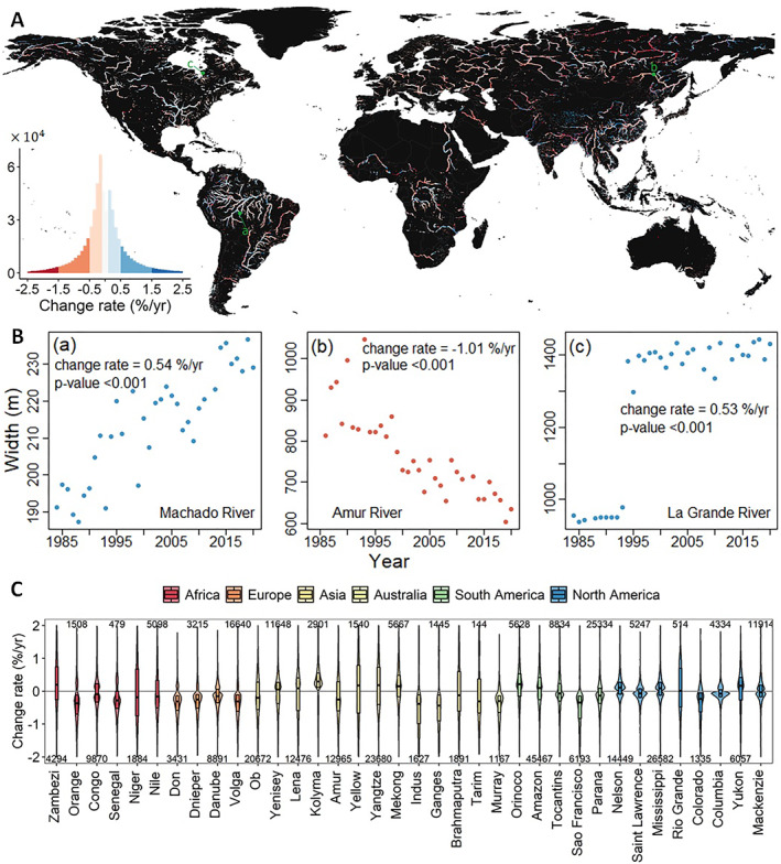
- About 85% of global rivers have width IQR <150 m; median and mean IQR are 34 and 96 m, respectively, with higher variability in Asia and West Africa (median IQR 70–210 m).
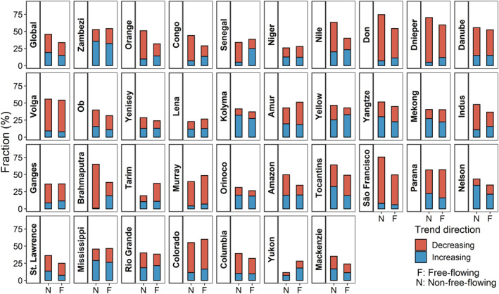
- Among 1.7 million river segments, 36.9% show a significant temporal trend (p < 0.05) in width during 1984–2020; 56.4% of these decrease and 43.6% increase, with 90% of slopes between −1.40% and +1.39%/yr. Non-free-flowing reaches show a higher fraction of significant trends (45.8%) than free-flowing reaches (33.6%), and 84% of non-free-flowing segments are impacted by dams/reservoirs.
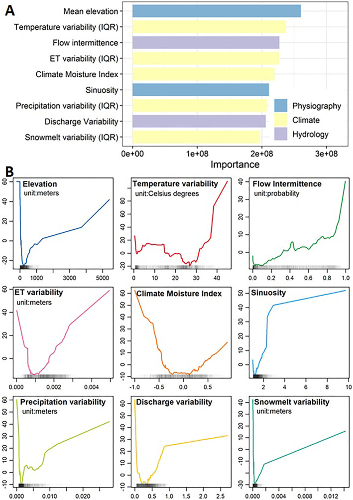
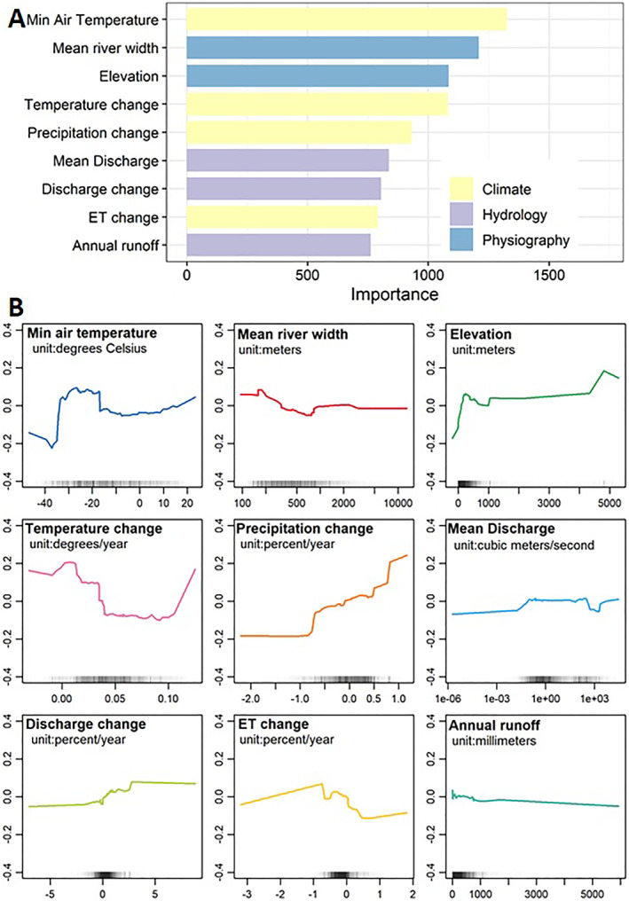
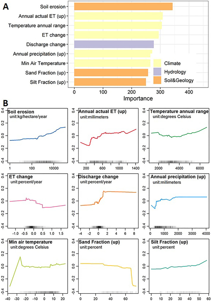
- Random Forest analysis indicates that free-flowing river width variability is most strongly explained by elevation, while free-flowing width trends are most strongly explained by minimum air temperature; for non-free-flowing rivers, soil/geology and anthropogenic parameters play more important roles.
Methods
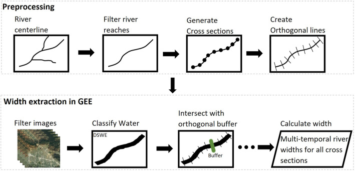
- Repeated river widths were extracted from Landsat 5, 7, and 8 images (1984–2020) in Google Earth Engine for MERIT Basin reaches wider than 90 m, using fixed orthogonal cross-sections, DSWE water classification, and automated screening for clouds, shadows, snow/ice, and inappropriate orthogonals.
- Temporal variability was quantified as IQR for cross-sections with at least 30 width measurements, and temporal trends were calculated from annual mean widths using the Mann-Kendall test for cross-sections with at least 15 years of observations; analysis was restricted to segments with all width measurements >90 m.
- Random Forest models (Ranger) used 117 environmental parameters in six categories, reduced to 59 subcategory representatives, with Accumulated Local Effects plots; separate models were run for free-flowing and non-free-flowing reaches, the latter defined by CSI <95 or location within 500 m of a GROD structure.
Limitations
- The paper states that fixed centerlines and orthogonals cannot account for river meandering, so high IQR may partly reflect channel meanders; fixed orthogonal length may miss extreme water extents and likely underestimates temporal variability; temporal resolution is low (2–8 measurements per year per cross-section on average); cloud screening (<25% coverage) trades data density for accuracy; and DSWE was validated only for sites across the US and Canada.
- The paper states that IQR is non-normalized and represents absolute rather than relative variability; environmental parameters are mostly model simulations or reanalysis products whose uncertainties propagate into Random Forest results; the study did not explicitly investigate causal mechanisms; and existing global anthropogenic data omit many dams/levees and may not fully represent human impacts.
- The text makes evident that the Random Forest results are correlational and that reach-scale aggregation of cross-sectional widths may introduce uncertainty due to uneven data availability within reaches, which the paper acknowledges.
Model-written summary. Check it against the paper before relying on it.
Integrity signals
Registry
Cites
Statistics
Figures


Verification
Claims the paper makes
0 Valid · 2 Not valid · 33 Not checked · 153 Own results and interpretations
A result the paper reports from its own data — it cites no other source for it, so there is none to check. The quote shows it is in the paper.
In the paper
“At the regional scale, rivers located in Asia (such as the Brahmaputra, Ganges, and Indus Rivers) and West Africa (e.g., the Niger River) show higher river width variabilities (median IQR ranges between 70 and 210 m) compared to other basins (Figures 2A and 2C).”
§ How Have Global River Widths Changed Over Time? > Results > Temporal Variations of Global River Width
plainstates an association- Asserted: passes — The authors put it forward as true.
- Checkable: passes — It can be checked against evidence.
- Load-bearing: unclear — It is unclear whether the paper’s conclusions depend on it.
- Based: passes — The paper gives a reason why it holds.
- Rests on an assumption not shown here.
A result the paper reports from its own data — it cites no other source for it, so there is none to check. The quote shows it is in the paper.
In the paper
“with 90% of the trend slopes ranging from −1.40% to +1.39%/yr.”
§ How Have Global River Widths Changed Over Time? > Results > Temporal Variations of Global River Width
plain- Asserted: passes — The authors put it forward as true.
- Checkable: passes — It can be checked against evidence.
- Load-bearing: unclear — It is unclear whether the paper’s conclusions depend on it.
- Based: passes — The paper gives a reason why it holds.
- Rests on an assumption not shown here.
A result the paper reports from its own data — it cites no other source for it, so there is none to check. The quote shows it is in the paper.
In the paper
“we found that non‐free‐flowing river reaches show a higher fraction (45.8%) of significant trends in river width than free‐flowing rivers (33.6%) (Figure 4).”
§ How Have Global River Widths Changed Over Time? > Results > Temporal Variations of Global River Width
plainstates an association- Asserted: passes — The authors put it forward as true.
- Checkable: passes — It can be checked against evidence.
- Load-bearing: passes — The paper’s conclusions depend on it.
- Based: passes — The paper gives a reason why it holds.
- Rests on an assumption not shown here.
A check of a cited source is scheduled, or we don’t hold its full text yet; the claim is checked once it runs.
In the paper
“we selected only river segments with all width measurements >90 m (i.e., the minimum width measurement >90 m) (Allen & Pavelsky, 2018), resulting in 2.7 million cross‐sections with a median river width of 439 m.”
§ How Have Global River Widths Changed Over Time? > Results
What the sources say
- Not checked yetcites Allen & Pavelsky, 2018 source
A check is scheduled.
plain- Asserted: passes — The authors put it forward as true.
- Checkable: passes — It can be checked against evidence.
- Load-bearing: passes — The paper’s conclusions depend on it.
- Based: passes — The paper gives a reason why it holds.
- Not checked yet
A result the paper reports from its own data — it cites no other source for it, so there is none to check. The quote shows it is in the paper.
In the paper
“Among the 36 largest river basins in the world, only one third (12/36) of them show more increasing than decreasing trends”
§ How Have Global River Widths Changed Over Time? > Results > Temporal Variations of Global River Width
plain- Asserted: passes — The authors put it forward as true.
- Checkable: passes — It can be checked against evidence.
- Load-bearing: unclear — It is unclear whether the paper’s conclusions depend on it.
- Based: passes — The paper gives a reason why it holds.
- Rests on 2 assumptions not shown here.
144 more claims
Create a free account to see all 188 claims and to verify the 32 references still open.
- Probably not a substantial claim. 19
- It may state two separate claims as one. 26
Self-check
Percentages, sums and reported differences re-computed from the paper’s own numbers.
Each contradiction between two passages listed here was confirmed by an independent check.
Rated minor: it would not touch a result — a value no result rests on, a p-value that stays on the same side of the significance level, or a conflict that is clerical, resolved elsewhere in the paper, or outside its own findings.
In the paper
§ How Have Global River Widths Changed Over Time? > Results > Temporal Variations of Global River Width
“Dam/reservoir impacts are dominant in the non‐free‐flowing rivers: 84% of these river segments are impacted by dams/reservoirs (Figure S4 in Supporting Information S1).”
§ How Have Global River Widths Changed Over Time? > Discussion
“We are encouraged that our results are broadly similar between normalized and non‐normalized metrics (Figures 2 and S4 in Supporting Information S1).”
Citations
Cites
Breiman, L. (2001) · Machine Learning · doi:10.1023/a:1010933404324 · Cited by 133,538
High-resolution mapping of global surface water and its long-term changes
Pekel, J.-F., Cottam, A., Gorelick, N., & Belward, A. S. (2016) · Nature · doi:10.1038/nature20584 · Cited by 5,513
SoilGrids250m: Global gridded soil information based on machine learning
Hengl, T., Mendes de Jesus, J., Heuvelink, G. B. M., Ruiperez Gonzalez, M., Kilibarda, M., Blagotić, A., Shangguan, W., Wright, M. N., Geng, X., Bauer-Marschallinger, B., et al. (2017) · PLOS ONE · doi:10.1371/journal.pone.0169748 · Cited by 4,733
Global hydrological cycles and world water resources
Oki, T., & Kanae, S. (2006) · Science · doi:10.1126/science.1128845 · Cited by 4,392 · cited 1×
“…impact humans and the environment by providing water/energy supply, aquatic habitats, transportation corridors, and geohydrological/biochemical connections with the atmosphere, land, and ocean (Feng et al., 2020; Gernaat et al., 2017; Oki & Kanae, 2006; Raymond et al., 2013; Syvitski et al., 2005).”
Backgroundranger: A Fast Implementation of Random Forests for High Dimensional Data in C++ and R
Wright, M. N., & Ziegler, A. (2017) · Journal of Statistical Software · doi:10.18637/jss.v077.i01 · Cited by 3,340
The hydraulic geometry of stream channels and some physiographic implications
Leopold, L. B., & Maddock, T. (1953) · Professional Paper · doi:10.3133/pp252 · Cited by 2,966
Impact of Humans on the Flux of Terrestrial Sediment to the Global Coastal Ocean
Syvitski, J. P. M., Vörösmarty, C. J., Kettner, A. J., & Green, P. (2005) · Science · doi:10.1126/science.1109454 · Cited by 2,818
Global carbon dioxide emissions from inland waters
Raymond, P. A., Hartmann, J., Lauerwald, R., Sobek, S., McDonald, C., Hoover, M., Butman, D., Striegl, R., Mayorga, E., Humborg, C., et al. (2013) · Nature · doi:10.1038/nature12760 · Cited by 2,553
Mapping the world’s free-flowing rivers
Grill, G., Lehner, B., Thieme, M., Geenen, B., Tickner, D., Antonelli, F., Babu, S., Borrelli, P., Cheng, L., Crochetiere, H., et al. (2019) · Nature · doi:10.1038/s41586-019-1111-9 · Cited by 2,473
A global boom in hydropower dam construction
Zarfl, C., Lumsdon, A. E., Berlekamp, J., Tydecks, L., & Tockner, K. (2015) · Aquatic Sciences · doi:10.1007/s00027-014-0377-0 · Cited by 2,181 · cited 1×
“Such infrastructure is likely becoming more common in populated areas, for example, the Amazon, Ganges–Brahmaputra, and Yangtze river basins (Zarfl et al., 2015), which could result in river width changes but was not represented here.”
Background
Cited by
Satellites reveal hotspots of global river extent change
Wu, Q., Ke, L., Wang, J., Pavelsky, T. M., Allen, G. H., Sheng, Y., Duan, X., Zhu, Y., Wu, J., Wang, L., et al. (2023) · Nature Communications · doi:10.1038/s41467-023-37061-3 · Cited by 140
Self-citationZhang, T., Li, D., East, A. E., Kettner, A. J., Best, J., Ni, J., & Lu, X. (2023) · Science Advances · doi:10.1126/sciadv.adi5019 · Cited by 115
More flow upstream and less flow downstream: The changing form and function of global rivers
Feng, D., & Gleason, C. J. (2024) · Science · doi:10.1126/science.adl5728 · Cited by 79
Self-citationLeaving a plastic legacy: Current and future scenarios for mismanaged plastic waste in rivers
Nyberg, B., Harris, P. T., Kane, I., & Maes, T. (2023) · The Science of The Total Environment · doi:10.1016/j.scitotenv.2023.161821 · Cited by 75
Global scale analysis on the extent of river channel belts
Nyberg, B., Henstra, G. A., Gawthorpe, R. L., Ravnås, R., & Ahokas, J. (2023) · Nature Communications · doi:10.1038/s41467-023-37852-8 · Cited by 62
Metadata
- Authors
- Feng, D., Gleason, C. J., Yang, X., Allen, G. H., & Pavelsky, T. M.
- Affiliations
- University of Cincinnati (US)
- University of Massachusetts Amherst (US)
- University of North Carolina at Chapel Hill (US)
- Virginia Tech (US)
- Corresponding author
- Feng, Dongmei
- Venue
- Water Resources Research
- Publisher
- American Geophysical Union (AGU)
- Published
- 2022-08
- Volume
- 58
- Issue
- 8
- Pages
- e2021WR031712-e2021WR031712
- ISSN
- 0043-1397 (ISSN-L)
- 1944-7973
- PMC
- PMC9541693
- OpenAlex
- W4293063191
- Cited by
- 70
- References
- 64
- Citations by year
- 2026: 23 · 2025: 18 · 2024: 19 · 2023: 10
- FWCI
- 6.86
- Type
- journal article
- Language
- en
- Open access
- hybrid
- doi.org
- Licence
- Locations
- Water Resources Research (publishedVersion, cc-by-nc-nd)
- PubMed (publishedVersion)
- PubMed Central (publishedVersion, cc-by-nc-nd)
- Funders
- National Aeronautics and Space Administration (80NSSC18K0741, 80NSSC21K0977, 80NSSC22K0987)
- California Institute of Technology
- Topics
- Physical Sciences › Earth and Planetary Sciences › Earth-Surface Processes › Hydrology and Sediment Transport Processes
- Physical Sciences › Environmental Science › Water Science and Technology › Hydrology and Watershed Management Studies
- Physical Sciences › Environmental Science › Global and Planetary Change › Flood Risk Assessment and Management
- Keywords
- river width, free-flowing rivers, anthropogenic impacts on rivers, soil conditions, river dynamics
About these checks
Registry, retraction, Cites and statistics results are computed, not judged, with one exception: a printed reference that no index lists is read once by a model before it counts as a citation error. Claims are extracted by a model and kept only when their quote appears verbatim in the text; each cited source is then checked, with a model’s help, for whether it says what the claim relies on. Those verdicts can be wrong — read the claim’s quote and the cited source before relying on one.
A language model drew the claims from the paper on 2026-11-18, under version 3 of the claim definition (model deepseek-v4.1-flash, prompt extract-v3).
A second model labelled each claim on 2026-11-18 (model jev-1.13-20260917, definition revision gold-guideline-v0.2).
Statistics and arithmetic are recomputed, not judged.
Confidence bands are shown only for fields calibrated on our annotated test set. None is calibrated yet, so no band is shown.
What counts as a claim ›How we measure confidence ›How we check this ›
Are you an author, or do you see a problem with this page? Request a review
How to cite
Cite CoChat for the checks on this page, and the paper for its own findings.
- This page
- CoChat. (2026). Citation check: How Have Global River Widths Changed Over Time? https://app.cochat.ai/papers/10.1029/2021wr031712
- The paper
- Feng, D., Gleason, C. J., Yang, X., Allen, G. H., & Pavelsky, T. M. (2022). How Have Global River Widths Changed Over Time? Water Resources Research. https://doi.org/10.1029/2021wr031712
Data sources
Bibliographic data: Semantic Scholar, OpenAlex, Crossref.
Contains information from the Semantic Scholar Academic Graph Datasets, made available under the ODC Attribution License (ODC-BY 1.0).
Semantic Scholar’s data is described in: Kinney, R., et al. (2023). The Semantic Scholar Open Data Platform. arXiv:2301.10140.
