

The DOI matches its Crossref record; 85 of the 89 references it cites were found in a registry or an index.
SoilGrids250m: Global gridded soil information based on machine learning
Open accessAbstract
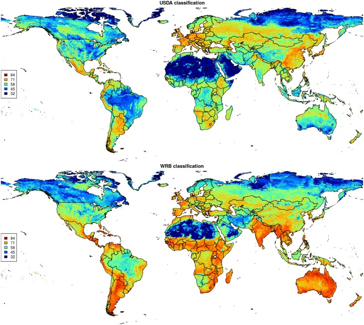
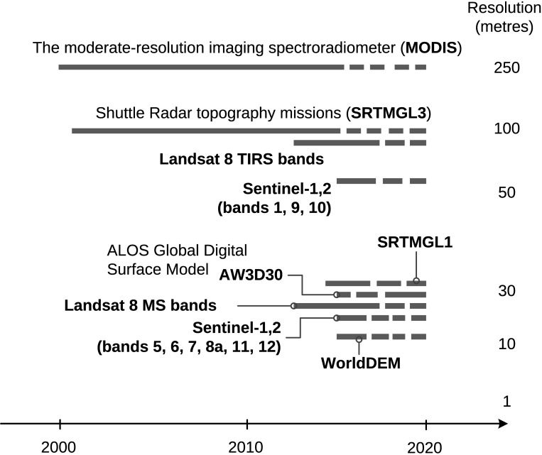
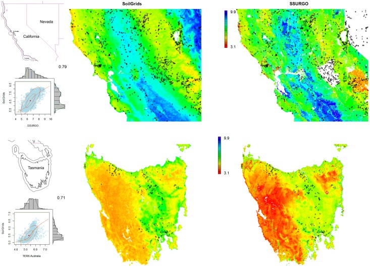
This paper describes the technical development and accuracy assessment of the most recent and improved version of the SoilGrids system at 250m resolution (June 2016 update). SoilGrids provides global predictions for standard numeric soil properties (organic carbon, bulk density, Cation Exchange Capacity (CEC), pH, soil texture fractions and coarse fragments) at seven standard depths (0, 5, 15, 30, 60, 100 and 200 cm), in addition to predictions of depth to bedrock and distribution of soil classes based on the World Reference Base (WRB) and USDA classification systems (ca. 280 raster layers in total). Predictions were based on ca. 150,000 soil profiles used for training and a stack of 158 remote sensing-based soil covariates (primarily derived from MODIS land products, SRTM DEM derivatives, climatic images and global landform and lithology maps), which were used to fit an ensemble of machine learning methods-random forest and gradient boosting and/or multinomial logistic regression-as implemented in the R packages ranger, xgboost, nnet and caret. The results of 10-fold cross-validation show that the ensemble models explain between 56% (coarse fragments) and 83% (pH) of variation with an overall average of 61%. Improvements in the relative accuracy considering the amount of variation explained, in comparison to the previous version of SoilGrids at 1 km spatial resolution, range from 60 to 230%. Improvements can be attributed to: (1) the use of machine learning instead of linear regression, (2) to considerable investments in preparing finer resolution covariate layers and (3) to insertion of additional soil profiles. Further development of SoilGrids could include refinement of methods to incorporate input uncertainties and derivation of posterior probability distributions (per pixel), and further automation of spatial modeling so that soil maps can be generated for potentially hundreds of soil variables. Another area of future research is the development of methods for multiscale merging of SoilGrids predictions with local and/or national gridded soil products (e.g. up to 50 m spatial resolution) so that increasingly more accurate, complete and consistent global soil information can be produced. SoilGrids are available under the Open Data Base License.
Overview
The claims and statistics of this paper haven’t been checked yet.
Free: it reads the open-access text and checks the first 5 claims that cite a source we can check. Create a free account to check every claim.
Integrity signals
Registry
Cites
Statistics
Figures






Verification
Claims the paper makes
The claims and statistics of this paper haven’t been checked yet.
Free: it reads the open-access text and checks the first 5 claims that cite a source we can check. Create a free account to check every claim.
Claims other papers make about this one
Each is checked against this paper’s own text: does it say what the citing paper says it does?
The source backs part of the claim, not all of it — or backs it for a different population, condition or comparison.
In the citing paper
“These uncertainties are mostly due to the uneven distribution and overall scarcity of field data for modelling and validating carbon stocks in the biomass and soil 27,64,65 .”
From Global priority areas for ecosystem restoration (2020) · cites this paper as [65]
Experimental — accuracy not yet measured
Self-check
Percentages, sums and reported differences re-computed from the paper’s own numbers.
The self-check needs the paper’s full text.
Citations
Cites
XGBoost: A Scalable Tree Boosting System
Chen, T., & Guestrin, C. (2016) · Proceedings of the 22nd ACM SIGKDD International Conference on Knowledge Discovery and Data Mining · doi:10.1145/2939672.2939785 · Cited by 54,569
Modern Applied Statistics with S
Venables, W. N., & Ripley, B. D. (2002) · Statistics and Computing · doi:10.1007/978-0-387-21706-2 · Cited by 24,305
Very high resolution interpolated climate surfaces for global land areas
Hijmans, R. J., Cameron, S. E., Parra, J. L., Jones, P. G., & Jarvis, A. (2005) · International Journal of Climatology · doi:10.1002/joc.1276 · Cited by 19,825
Total Carbon, Organic Carbon, and Organic Matter
Nelson, D. W., & Sommers, L. E. (1982) · Agronomy Monographs · doi:10.2134/agronmonogr9.2.2ed.c29 · Cited by 9,978
Building Predictive Models in R Using the caret Package
Kuhn, M. (2008) · Journal of Statistical Software · doi:10.18637/jss.v028.i05 · Cited by 8,863
Weighted kappa: nominal scale agreement provision for scaled disagreement or partial credit
Cohen, J. (1968) · Psychological Bulletin · doi:10.1037/h0026256 · Cited by 8,736
Kuhn, M., & Johnson, K. (2013) · doi:10.1007/978-1-4614-6849-3 · Cited by 6,788
Communication in the presence of noise
Shannon, C. E. (1949) · Proceedings of the IRE · doi:10.1109/jrproc.1949.232969 · Cited by 6,539
Anonim, A. (2010) · Cited by 4,945
Communication In The Presence Of Noise
Shannon, C. E. (1998) · Proceedings of the IEEE · doi:10.1109/jproc.1998.659497 · Cited by 4,804
Research works printed but not linked: 5
- D Arrouays, 2014, Soil carbon. vol. 125 of Advances in Agronomy, 93
- SA Lei, 1998, Soil Properties of the Kelso Sand Dunes in the Mojave Desert, The Southwestern Naturalist, 43, 47
- Huffman GJ, Bolvin DT. GPCP version 2 combined precipitation data set documentation. vol. 1. Laboratory for Atmospheres, NASA Goddard Space Flight Center and Science Systems and Applications; 2009.
- Kempen B. Updating soil information with digital soil mapping [PhD thesis]. Wageningen University. Wageningen; 2011. Available from: http://edepot.wur.nl/187198.
- Eberhardt E. Deriving WRB soil types using National German Soil Survey Guidelines. In: NCSS National Conference. NCSS Standards. Asheville, NC: United States Department of Agriculture USDA-NRCS; 2011. p. 1–2.
Cited by
Deep learning and process understanding for data-driven Earth system science
Reichstein, M., Camps-Valls, G., Stevens, B., Jung, M., Denzler, J., Carvalhais, N., & Prabhat (2019) · Nature · doi:10.1038/s41586-019-0912-1 · Cited by 5,673
SoilGrids 2.0: producing soil information for the globe with quantified spatial uncertainty
Poggio, L., de Sousa, L. M., Batjes, N. H., Heuvelink, G. B. M., Kempen, B., Ribeiro, E., & Rossiter, D. (2021) · SOIL · doi:10.5194/soil-7-217-2021 · Cited by 2,333
Self-citationA global atlas of the dominant bacteria found in soil
Delgado-Baquerizo, M., Oliverio, A. M., Brewer, T. E., Benavent-González, A., Eldridge, D. J., Bardgett, R. D., Maestre, F. T., Singh, B. K., & Fierer, N. (2018) · Science · doi:10.1126/science.aap9516 · Cited by 2,301
The global tree restoration potential
Bastin, J.-F., Finegold, Y., Garcia, C., Mollicone, D., Rezende, M., Routh, D., Zohner, C. M., & Crowther, T. W. (2019) · Science · doi:10.1126/science.aax0848 · Cited by 2,197
Rainfall–runoff modelling using Long Short-Term Memory (LSTM) networks
(2018) · doi:10.5194/hess-22-6005-2018 · Cited by 2,114
Metadata
- Authors
- Hengl, T., Mendes de Jesus, J., Heuvelink, G. B. M., Ruiperez Gonzalez, M., Kilibarda, M., Blagotić, A., Shangguan, W., Wright, M. N., Geng, X., Bauer-Marschallinger, B., Guevara, M. A., Vargas, R., MacMillan, R. A., Batjes, N. H., Leenaars, J. G. B., Ribeiro, E., Wheeler, I., Mantel, S., & Kempen, B.
- Affiliations
- ISRIC - World Soil Information (NL)
- University of Belgrade (RS)
- Sun Yat-sen University (CN)
- University of Lübeck (DE)
- Agriculture and Agri-Food Canada (CA)
- TU Wien (AT)
- University of Delaware (US)
- ORCID
- Venue
- PLOS ONE
- Publisher
- Public Library of Science (PLoS)
- Published
- 2017-02-16
- Volume
- 12
- Issue
- 2
- Pages
- e0169748
- ISSN
- 1932-6203 (ISSN-L)
- PMC
- PMC5313206
- OpenAlex
- W2588003345
- Cited by
- 4,733
- References
- 89
- Citations by year
- 2026: 591 · 2025: 654 · 2024: 610 · 2023: 634 · 2022: 669 · 2021: 672 · 2020: 402 · 2019: 265 · 2018: 173 · 2017: 56
- FWCI
- 137.14
- Type
- journal article
- Language
- en
- Open access
- gold
- doi.org
- Licence
- Locations
- PLoS ONE (publishedVersion, cc-by)
- PubMed Central (publishedVersion, cc-by)
- PubMed (publishedVersion)
- RePEc: Research Papers in Economics (submittedVersion)
- DOAJ (DOAJ: Directory of Open Access Journals) (submittedVersion)
- GraFar (University of Belgrade, Faculty of Civil Engineering) (submittedVersion, cc-by)
- Socio-Environmental Systems Modeling (submittedVersion, cc-by)
- Data Archiving and Networked Services (DANS) (submittedVersion, other-oa)
- Topics
- Life Sciences › Agricultural and Biological Sciences › Soil Science › Soil Geostatistics and Mapping
- Physical Sciences › Environmental Science › Environmental Engineering › Soil Moisture and Remote Sensing
- Physical Sciences › Environmental Science › Management, Monitoring, Policy and Law › Soil and Land Suitability Analysis
- Keywords
- SoilGrids, soil properties, soil organic carbon, soil bulk density, cation exchange capacity, soil pH, soil texture, coarse fragments, bedrock depth, soil classification, USDA soil classification, MODIS, random forest, gradient boosting, multinomial logistic regression, ensemble learning, accuracy assessment, soil mapping
- MeSH terms
- Machine Learning, Algorithms, Conservation of Natural Resources, Environmental Monitoring, Humans, Models, Theoretical, Soil, Geographic Information Systems
About these checks
Registry, retraction, Cites and statistics results are computed, not judged, with one exception: a printed reference that no index lists is read once by a model before it counts as a citation error. Claims are extracted by a model and kept only when their quote appears verbatim in the text; each cited source is then checked, with a model’s help, for whether it says what the claim relies on. Those verdicts can be wrong — read the claim’s quote and the cited source before relying on one.
Statistics and arithmetic are recomputed, not judged.
Confidence bands are shown only for fields calibrated on our annotated test set. None is calibrated yet, so no band is shown.
What counts as a claim ›How we measure confidence ›How we check this ›
Are you an author, or do you see a problem with this page? Request a review
How to cite
Cite CoChat for the checks on this page, and the paper for its own findings.
- This page
- CoChat. (2026). Citation check: SoilGrids250m: Global gridded soil information based on machine learning. https://app.cochat.ai/papers/10.1371/journal.pone.0169748
- The paper
- Hengl, T., Mendes de Jesus, J., Heuvelink, G. B. M., Ruiperez Gonzalez, M., Kilibarda, M., Blagotić, A., Shangguan, W., Wright, M. N., Geng, X., Bauer-Marschallinger, B., Guevara, M. A., Vargas, R., MacMillan, R. A., Batjes, N. H., Leenaars, J. G. B., Ribeiro, E., Wheeler, I., Mantel, S., & Kempen, B. (2017). SoilGrids250m: Global gridded soil information based on machine learning. PLOS ONE. https://doi.org/10.1371/journal.pone.0169748
Data sources
Bibliographic data: Semantic Scholar, OpenAlex, Crossref.
Contains information from the Semantic Scholar Academic Graph Datasets, made available under the ODC Attribution License (ODC-BY 1.0).
Semantic Scholar’s data is described in: Kinney, R., et al. (2023). The Semantic Scholar Open Data Platform. arXiv:2301.10140.
