Student or educator? Sign up with your school email and get 6 months of Pro free.
CoChat

The DOI matches its Crossref record; 64 of the 64 references it cites were found in a registry or an index.

Unsupervised deep learning identifies semantic disentanglement in single inferotemporal face patch neurons

Open access
Higgins, Irina, Chang, Le, Langston, Victoria, Hassabis, Demis, Summerfield, Christopher, Tsao, Doris, Botvinick, Matthew · 2021 · Nature Communications

Abstract

In order to better understand how the brain perceives faces, it is important to know what objective drives learning in the ventral visual stream. To answer this question, we model neural responses to faces in the macaque inferotemporal (IT) cortex with a deep self-supervised generative model, β -VAE, which disentangles sensory data into interpretable latent factors, such as gender or age. Our results demonstrate a strong correspondence between the generative factors discovered by β -VAE and those coded by single IT neurons, beyond that found for the baselines, including the handcrafted state-of-the-art model of face perception, the Active Appearance Model, and deep classifiers. Moreover, β -VAE is able to reconstruct novel face images using signals from just a handful of cells. Together our results imply that optimising the disentangling objective leads to representations that closely resemble those in the IT at the single unit level. This points at disentangling as a plausible learning objective for the visual brain.

Overview

The claims and statistics of this paper haven’t been checked yet.

Free: it reads the open-access text and checks the first 5 claims that cite a source we can check. Create a free account to check every claim.

A few free checks a day · papers already verified open instantly · results are public

Integrity signals

Registry

Crossref · 10.1038/s41467-021-26751-5

Cites

64 of 64 references verified0 citation errors · 0 not checkable

Statistics

Figures

Fig. 1 Disentangled representation learning. a Latent traversals used to visualise the semantic meaning encoded by single disentangled latent units of a trained model. In each row the value of a single latent unit is varied between −3 and 3, while the other units are fixed. The resulting effect on the reconstruction is visualised. Each column represents a different model trained to disentangle a different dataset. Chair and face images in the leftmost two traversals are reproduced with the permission of Lee et al.19. Traversals of 3D scenes are reproduced with the permission of Burgess et al.18. b Schematic representation of a self-supervised deep neural network. The encoder maps the input image into a low-dimensional latent representation, which is used by the decoder to reconstruct the original image. Blue indicates trainable neural network units that are free to represent anything. Pink indicates latent representation units that are compared to neurons. CNN, convolutional neural network. FC, fully connected neural network. Face image reproduced with permission from Gao et al.57. c Latent traversals of eight units of a β-VAE model trained to disentangle 2100 natural face images. The initial values of all latent units were obtained by encoding the same input image.
Fig. 1 Disentangled representation learning. a Latent traversals used to visualise the semantic meaning encoded by single disentangled latent units of a trained model. In each row the value of a single latent unit is varied between −3 and 3, while the other units are fixed. The resulting effect on the reconstruction is visualised. Each column represents a different model trained to disentangle a different dataset. Chair and face images in the leftmost two traversals are reproduced with the permission of Lee et al.19. Traversals of 3D scenes are reproduced with the permission of Burgess et al.18. b Schematic representation of a self-supervised deep neural network. The encoder maps the input image into a low-dimensional latent representation, which is used by the decoder to reconstruct the original image. Blue indicates trainable neural network units that are free to represent anything. Pink indicates latent representation units that are compared to neurons. CNN, convolutional neural network. FC, fully connected neural network. Face image reproduced with permission from Gao et al.57. c Latent traversals of eight units of a β-VAE model trained to disentangle 2100 natural face images. The initial values of all latent units were obtained by encoding the same input image.CC BY · PubMed Central
Fig. 2 Responses of single neurons are well explained by single disentangled latent units. a Coronal section showing the location of fMRI-identified face patches in two primates, with patch AM circled in red. Dark black lines, electrodes. Reproduced with permission from Chang et al.6. b Explained variance of single neuron responses to 2100 faces. Response variance in single neurons is explained primarily by single disentangled units encoding different semantically meaningful information (insets, latent traversals as in Fig. 1a, c). Source data are provided as a Source Data file.
Fig. 2 Responses of single neurons are well explained by single disentangled latent units. a Coronal section showing the location of fMRI-identified face patches in two primates, with patch AM circled in red. Dark black lines, electrodes. Reproduced with permission from Chang et al.6. b Explained variance of single neuron responses to 2100 faces. Response variance in single neurons is explained primarily by single disentangled units encoding different semantically meaningful information (insets, latent traversals as in Fig. 1a, c). Source data are provided as a Source Data file.CC BY · PubMed Central
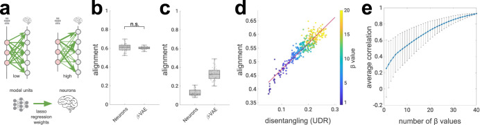
Fig. 3 Strong alignment between single neurons and disentangled units. a Schematic of alignment score29, 63. Green arrows, lasso regression weights obtained from predicting neural responses from model units (thickness indicates weight magnitude). High alignment scores are obtained when per-neuron regression weights have low entropy (one strong weight); high entropy (all incoming weights are of equal magnitude) results in low alignment scores. b β-VAE alignment scores match the ceiling provided by subsets of neurons (p = 0.4345, two-sided Welsch’s t-test). Circles, alignment per model (n = 51) or neuron subsets (n = 50). Boxplot centre is median, box extends to 25th and 75th percentiles, whiskers extend to the most extreme data that are not considered outliers, outliers are plotted individually. Source data are provided as a Source Data file. c Alignment scores per model (n = 51) or neuron subsets (n = 50) against artificial neural responses (linear recombination of original neural responses). Boxplot centre is median, box extends to 25th and 75th percentiles, whiskers extend to the most extreme data that are not considered outliers, outliers are plotted individually. Source data are provided as a Source Data file. d Alignment scores correlate with the disentanglement quality of latent units obtained from 400 β-VAE models trained with different β values (indicated by colour). UDR, Unsupervised Disentanglement Ranking31, measures the quality of disentanglement, higher is better. Red line, least squares fit (r = 0.96, Pearson correlation). Source data are provided as a Source Data file. e Running correlation between UDR and alignment scores across subsets of models. Models in each subset were trained with different β values, with the number of β values in each subset indicated on the x-axis. Rightmost circle, Pearson correlation across 400 β-VAE models, spanning 40 β values as reported in (d). Leftmost circle, average across 40 Pearson correlations, each calculated with 10 models with a single β value. Bars, standard deviation. Source data are provided as a Source Data file.
Fig. 3 Strong alignment between single neurons and disentangled units. a Schematic of alignment score29, 63. Green arrows, lasso regression weights obtained from predicting neural responses from model units (thickness indicates weight magnitude). High alignment scores are obtained when per-neuron regression weights have low entropy (one strong weight); high entropy (all incoming weights are of equal magnitude) results in low alignment scores. b β-VAE alignment scores match the ceiling provided by subsets of neurons (p = 0.4345, two-sided Welsch’s t-test). Circles, alignment per model (n = 51) or neuron subsets (n = 50). Boxplot centre is median, box extends to 25th and 75th percentiles, whiskers extend to the most extreme data that are not considered outliers, outliers are plotted individually. Source data are provided as a Source Data file. c Alignment scores per model (n = 51) or neuron subsets (n = 50) against artificial neural responses (linear recombination of original neural responses). Boxplot centre is median, box extends to 25th and 75th percentiles, whiskers extend to the most extreme data that are not considered outliers, outliers are plotted individually. Source data are provided as a Source Data file. d Alignment scores correlate with the disentanglement quality of latent units obtained from 400 β-VAE models trained with different β values (indicated by colour). UDR, Unsupervised Disentanglement Ranking31, measures the quality of disentanglement, higher is better. Red line, least squares fit (r = 0.96, Pearson correlation). Source data are provided as a Source Data file. e Running correlation between UDR and alignment scores across subsets of models. Models in each subset were trained with different β values, with the number of β values in each subset indicated on the x-axis. Rightmost circle, Pearson correlation across 400 β-VAE models, spanning 40 β values as reported in (d). Leftmost circle, average across 40 Pearson correlations, each calculated with 10 models with a single β value. Bars, standard deviation. Source data are provided as a Source Data file.CC BY · PubMed Central
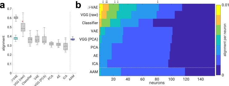
Fig. 4 Disentangled latent units align with single neurons better than baselines. a Alignment scores are significantly higher for the β-VAE than the baseline models and the “gold standard” provided by the AAM (all p < 0.01, two-sided Welsch’s t-test; VGG (raw) p = 7.4220e–06, Classifier p = 0.0, AAM p = 9.1757e–42, VAE p = 9.7811e–43, VGG (PCA) p = 1.9383e–35, PCA p = 0.0, AE p = 0.0, ICA p = 0.0). Circles, alignment per model (β-VAE, n = 51; VGG (raw), n = 22; Classifier, n = 64; VAE, Variational AutoEncoder36, n = 50; AE, AutoEncoder35, n = 50; VGG (PCA)32, n = 41; PCA, n = 41; ICA, n = 50; AAM, active appearance model3, n = 21). Red circle indicates VGG (raw) with all N = 4096 units from the last hidden layer. Teal boxplot—random baseline with sparseness matched to the 51 β-VAE models. Boxplot centre is median, box extends to 25th and 75th percentiles, whiskers extend to the most extreme data that are not considered outliers, outliers are plotted individually. Source data are provided as a Source Data file. b Per-neuron alignment scores. Scores are discretised into equally spaced bins. Scores in each row are arranged in descending order. The results from single models, chosen to have the median alignment score. VGG (raw) results are presented from the model that contained all N = 4096 units from the last hidden layer. Arrows point to neurons from Fig. 2b within the β-VAE alignment scores. Source data are provided as a Source Data file.
Fig. 4 Disentangled latent units align with single neurons better than baselines. a Alignment scores are significantly higher for the β-VAE than the baseline models and the “gold standard” provided by the AAM (all p < 0.01, two-sided Welsch’s t-test; VGG (raw) p = 7.4220e–06, Classifier p = 0.0, AAM p = 9.1757e–42, VAE p = 9.7811e–43, VGG (PCA) p = 1.9383e–35, PCA p = 0.0, AE p = 0.0, ICA p = 0.0). Circles, alignment per model (β-VAE, n = 51; VGG (raw), n = 22; Classifier, n = 64; VAE, Variational AutoEncoder36, n = 50; AE, AutoEncoder35, n = 50; VGG (PCA)32, n = 41; PCA, n = 41; ICA, n = 50; AAM, active appearance model3, n = 21). Red circle indicates VGG (raw) with all N = 4096 units from the last hidden layer. Teal boxplot—random baseline with sparseness matched to the 51 β-VAE models. Boxplot centre is median, box extends to 25th and 75th percentiles, whiskers extend to the most extreme data that are not considered outliers, outliers are plotted individually. Source data are provided as a Source Data file. b Per-neuron alignment scores. Scores are discretised into equally spaced bins. Scores in each row are arranged in descending order. The results from single models, chosen to have the median alignment score. VGG (raw) results are presented from the model that contained all N = 4096 units from the last hidden layer. Arrows point to neurons from Fig. 2b within the β-VAE alignment scores. Source data are provided as a Source Data file.CC BY · PubMed Central
Fig. 5 Disentangled latent units have better diversity and one-to-one correlation with neurons compared to baselines. a Schematic of average correlation ratio and average unit proportion scores. A good computational model for explaining responses of single neurons should allow each neuron (grey circle) to be decodable from a single latent unit (pink circle). Green lines are Lasso regression weights as in Fig. 3a. The response of each neuron should correlate strongly with the response of only one latent unit (grey bars) as measured by the average correlation ratio (higher is better). Different neurons should correlate strongly with diverse single latent units (red circles) as measured by the average unit proportion score (higher is better). b Average correlation ratio scores are significantly higher for the β-VAE than the baseline models and the AAM model (all p < 0.01; AAM p = 3.4626e–07, ICA p = 4.3804e–07, VGG (PCA) p = 2.9275e–15, PCA p = 1.8577e–15, VAE p = 5.7259e–13, AE p = 8.2339e–16, Classifier p = 7.8206e−55, VGG (raw) p = 1.4072e–26, two-sided Welsch’s t-test). Circles, average correlation ratio score per model (β-VAE, n = 51; VGG (raw), n = 22; Classifier, n = 64; VAE, Variational AutoEncoder36, n = 50; AE, AutoEncoder35, n = 50; VGG (PCA)32, n = 41; PCA, n = 41; ICA, n = 50; AAM, active appearance model3, n = 21). Boxplot centre is median, box extends to 25th and 75th percentiles, whiskers extend to the most extreme data that are not considered outliers, outliers are plotted individually. Source data are provided as a Source Data file. c Average unit proportion scores are significantly higher for the β-VAE than the baseline models and the AAM model (all p < 0.01; Classifier p = 4.5163e–10, AE p = 1.4289e–04, VAE p = 4.1792e–14, ICA p = 1.1129e–19, VGG (PCA) p = 1.7441e–19, PCA p = 3.5554e–19, AAM p = 1.8075e–09, VGG (raw) p = 1.2049e–08, two-sided Welsch’s t-test). Circles, average unit proportion score per model (β-VAE, n = 51; VGG (raw), n = 22; Classifier, n = 64; VAE36, n = 50; AE35, n = 50; VGG (PCA)32, n = 41; PCA, n = 41; ICA, n = 50; AAM3, n = 21). Boxplot centre is median, box extends to 25th and 75th percentiles, whiskers extend to the most extreme data that are not considered outliers, outliers are plotted individually. Source data are provided as a Source Data file.
Fig. 5 Disentangled latent units have better diversity and one-to-one correlation with neurons compared to baselines. a Schematic of average correlation ratio and average unit proportion scores. A good computational model for explaining responses of single neurons should allow each neuron (grey circle) to be decodable from a single latent unit (pink circle). Green lines are Lasso regression weights as in Fig. 3a. The response of each neuron should correlate strongly with the response of only one latent unit (grey bars) as measured by the average correlation ratio (higher is better). Different neurons should correlate strongly with diverse single latent units (red circles) as measured by the average unit proportion score (higher is better). b Average correlation ratio scores are significantly higher for the β-VAE than the baseline models and the AAM model (all p < 0.01; AAM p = 3.4626e–07, ICA p = 4.3804e–07, VGG (PCA) p = 2.9275e–15, PCA p = 1.8577e–15, VAE p = 5.7259e–13, AE p = 8.2339e–16, Classifier p = 7.8206e−55, VGG (raw) p = 1.4072e–26, two-sided Welsch’s t-test). Circles, average correlation ratio score per model (β-VAE, n = 51; VGG (raw), n = 22; Classifier, n = 64; VAE, Variational AutoEncoder36, n = 50; AE, AutoEncoder35, n = 50; VGG (PCA)32, n = 41; PCA, n = 41; ICA, n = 50; AAM, active appearance model3, n = 21). Boxplot centre is median, box extends to 25th and 75th percentiles, whiskers extend to the most extreme data that are not considered outliers, outliers are plotted individually. Source data are provided as a Source Data file. c Average unit proportion scores are significantly higher for the β-VAE than the baseline models and the AAM model (all p < 0.01; Classifier p = 4.5163e–10, AE p = 1.4289e–04, VAE p = 4.1792e–14, ICA p = 1.1129e–19, VGG (PCA) p = 1.7441e–19, PCA p = 3.5554e–19, AAM p = 1.8075e–09, VGG (raw) p = 1.2049e–08, two-sided Welsch’s t-test). Circles, average unit proportion score per model (β-VAE, n = 51; VGG (raw), n = 22; Classifier, n = 64; VAE36, n = 50; AE35, n = 50; VGG (PCA)32, n = 41; PCA, n = 41; ICA, n = 50; AAM3, n = 21). Boxplot centre is median, box extends to 25th and 75th percentiles, whiskers extend to the most extreme data that are not considered outliers, outliers are plotted individually. Source data are provided as a Source Data file.CC BY · PubMed Central
Fig. 6 Variance-explained results. a Schematic representation of linearly accessible information overlap between the population of neurons (green) and model representation (blue) corresponding to the different combinations of magnitudes of the encoding and decoding scores. b Ratio of total neuron population (n = 159) for which single β-VAE units explain more variance than X% of variance explained by the best baseline model (AAM, 50 units). See Supplementary Fig. 3 for more details. Source data are provided as a Source Data file. c Encoding variance explained. No significant difference is found between encoding variance explained by neuron subsets and AE, ICA, VAE, PCA and AAM (β-VAE p = 2.4689e–08, AAM p = 0.1211, VGG (PCA) p = 2.5055e–07, PCA p = 0.0174, Classifier p = 2.6311e–17, ICA p = 0.0185, AE p = 0.0368, VAE p = 0.0176, VGG (raw) p = 8.4568e–18, two-sided Welsch’s t-test). Circles, median explained variance across 159 neurons (β-VAE, n = 51; VGG (raw), n = 22; Classifier, n = 64; VAE, Variational AutoEncoder36, n = 50; AE, AutoEncoder35, n = 50; VGG (PCA)32, n = 41; PCA, n = 41; ICA, n = 50; AAM, active appearance model3, n = 21). Boxplot centre is median, box extends to 25th and 75th percentiles, whiskers extend to the most extreme data that are not considered outliers, outliers are plotted individually. Source data are provided as a Source Data file. d Decoding variance explained. β-VAE variance explained is statistically significantly different from all other models (all p < 0.01; AAM p = 7.6510e–07, VGG (PCA) p = 0.0, PCA p = 6.0566e–23, Classifier p = 0.0, ICA p = 2.8584e–20, AE p = 0.0164, VAE p = 1.1390e–12, VGG (raw) p = 0.0, two-sided Welsch’s t-test). Circles, median explained variance across model units (β-VAE, n = 51; VGG (raw), n = 22; Classifier, n = 64; VAE, Variational AutoEncoder36, n = 50; AE, AutoEncoder35, n = 50; VGG (PCA)32, n = 41; PCA, n = 41; ICA, n = 50; AAM, active appearance model3, n = 21). Boxplot centre is median, box extends to 25th and 75th percentiles, whiskers extend to the most extreme data that are not considered outliers, outliers are plotted individually. Source data are provided as a Source Data file.
Fig. 6 Variance-explained results. a Schematic representation of linearly accessible information overlap between the population of neurons (green) and model representation (blue) corresponding to the different combinations of magnitudes of the encoding and decoding scores. b Ratio of total neuron population (n = 159) for which single β-VAE units explain more variance than X% of variance explained by the best baseline model (AAM, 50 units). See Supplementary Fig. 3 for more details. Source data are provided as a Source Data file. c Encoding variance explained. No significant difference is found between encoding variance explained by neuron subsets and AE, ICA, VAE, PCA and AAM (β-VAE p = 2.4689e–08, AAM p = 0.1211, VGG (PCA) p = 2.5055e–07, PCA p = 0.0174, Classifier p = 2.6311e–17, ICA p = 0.0185, AE p = 0.0368, VAE p = 0.0176, VGG (raw) p = 8.4568e–18, two-sided Welsch’s t-test). Circles, median explained variance across 159 neurons (β-VAE, n = 51; VGG (raw), n = 22; Classifier, n = 64; VAE, Variational AutoEncoder36, n = 50; AE, AutoEncoder35, n = 50; VGG (PCA)32, n = 41; PCA, n = 41; ICA, n = 50; AAM, active appearance model3, n = 21). Boxplot centre is median, box extends to 25th and 75th percentiles, whiskers extend to the most extreme data that are not considered outliers, outliers are plotted individually. Source data are provided as a Source Data file. d Decoding variance explained. β-VAE variance explained is statistically significantly different from all other models (all p < 0.01; AAM p = 7.6510e–07, VGG (PCA) p = 0.0, PCA p = 6.0566e–23, Classifier p = 0.0, ICA p = 2.8584e–20, AE p = 0.0164, VAE p = 1.1390e–12, VGG (raw) p = 0.0, two-sided Welsch’s t-test). Circles, median explained variance across model units (β-VAE, n = 51; VGG (raw), n = 22; Classifier, n = 64; VAE, Variational AutoEncoder36, n = 50; AE, AutoEncoder35, n = 50; VGG (PCA)32, n = 41; PCA, n = 41; ICA, n = 50; AAM, active appearance model3, n = 21). Boxplot centre is median, box extends to 25th and 75th percentiles, whiskers extend to the most extreme data that are not considered outliers, outliers are plotted individually. Source data are provided as a Source Data file.CC BY · PubMed Central
Fig. 7 Reconstructing novel faces from single neurons. a Responses of 159 neurons (grey circles) in face-patch area AM were recorded while two primates viewed 62 novel faces. One-to-one match was found between each model unit (pink circles) and a corresponding single neuron. Linear regression (blue arrow) was used to decode the responses of each individual model latent unit (pink circles) from the activations of its corresponding single neuron. The pre-trained model decoder was used to reconstruct the novel face. Face image reproduced with permission from Chang et al.6. b Cosine distance between real standardised latent unit responses and those decoded from single neurons are significantly smaller for β-VAE compared to baseline models and the “gold standard” provided by the AAM model (all p < 0.05, single-sided Welsch’s t-test; AE p = 0.0195, VAE p = 1.0596e–14, PCA p = 4.0370e–25, ICA p = 1.5758e–12, VGG (PCA) p = 5.0467e–24, Classifier p = 0.0, AAM p = 2.3216e–14, VGG (raw) p = 4.8840e–20). Circles, median cosine distance per model (β-VAE, n = 51; VGG (raw), n = 22; Classifier, n = 64; VAE, Variational AutoEncoder36, n = 50; AE, AutoEncoder35, n = 50; VGG (PCA)32, n = 41; PCA, n = 41; ICA, n = 50; AAM, active appearance model3, n = 21). Boxplot centre is median, box extends to 25th and 75th percentiles, whiskers extend to the most extreme data that are not considered outliers, outliers are plotted individually. Source data are provided as a Source Data file. c β-VAE can decode and reconstruct novel faces from 12 matching single neurons. The reconstructions are better than those from the closest baselines, AE and VAE, which required 30 and 27 neurons for decoding, respectively. The β-VAE instance was chosen to have the best disentanglement quality as measured by the UDR score; AE and VAE instances were chosen to have the highest reconstruction accuracy on the training dataset. Face images reproduced with permission from Ma et al.53 and Phillips et al.55.
Fig. 7 Reconstructing novel faces from single neurons. a Responses of 159 neurons (grey circles) in face-patch area AM were recorded while two primates viewed 62 novel faces. One-to-one match was found between each model unit (pink circles) and a corresponding single neuron. Linear regression (blue arrow) was used to decode the responses of each individual model latent unit (pink circles) from the activations of its corresponding single neuron. The pre-trained model decoder was used to reconstruct the novel face. Face image reproduced with permission from Chang et al.6. b Cosine distance between real standardised latent unit responses and those decoded from single neurons are significantly smaller for β-VAE compared to baseline models and the “gold standard” provided by the AAM model (all p < 0.05, single-sided Welsch’s t-test; AE p = 0.0195, VAE p = 1.0596e–14, PCA p = 4.0370e–25, ICA p = 1.5758e–12, VGG (PCA) p = 5.0467e–24, Classifier p = 0.0, AAM p = 2.3216e–14, VGG (raw) p = 4.8840e–20). Circles, median cosine distance per model (β-VAE, n = 51; VGG (raw), n = 22; Classifier, n = 64; VAE, Variational AutoEncoder36, n = 50; AE, AutoEncoder35, n = 50; VGG (PCA)32, n = 41; PCA, n = 41; ICA, n = 50; AAM, active appearance model3, n = 21). Boxplot centre is median, box extends to 25th and 75th percentiles, whiskers extend to the most extreme data that are not considered outliers, outliers are plotted individually. Source data are provided as a Source Data file. c β-VAE can decode and reconstruct novel faces from 12 matching single neurons. The reconstructions are better than those from the closest baselines, AE and VAE, which required 30 and 27 neurons for decoding, respectively. The β-VAE instance was chosen to have the best disentanglement quality as measured by the UDR score; AE and VAE instances were chosen to have the highest reconstruction accuracy on the training dataset. Face images reproduced with permission from Ma et al.53 and Phillips et al.55.CC BY · PubMed Central
Fig. 8 Schematic of model architectures. Blue, trainable neural network units free to represent anything. Pink, latent representation units used for comparison with neurons in response to 2100 face images. Grey, units representing class probabilities. CNN, convolutional neural network. FC, fully connected neural network. N, number of latent units. a Self-supervised models — β-VAE17, autoencoder (AE)35 and variational autoencoder (VAE)36, 58. Models were trained on the mirror flipped versions of the 2100 faces presented to the primates. Face image reproduced with permission from Gao et al.57. b Classifier baseline. Encoder network, same as in (a). Model trained to differentiate between unique 2100 face identities using mirror flipped versions of the 2100 faces augmented with 5 × 5 pixel translations. Face image reproduced with permission from Gao et al.57. c VGG baseline32. Encoder network has larger and deeper CNN and FC modules than in (a) and (b). Representation dimensionality is reduced to match other models either by a projection on the first N principal components (PCs) (VGG (PCA)), or by taking a random subset of N units without replacement (VGG (raw)). VGG was trained to differentiate between 2622 unique faces using a face dataset32 unrelated to the 2100 faces presented to the primates. Face image is representative of the images used to train the model and is reproduced with permission from Liu et al.52. d Active appearance model (AAM)3. Keypoints were manually placed on the 2100 face images. First N/2 PCs over the keypoint locations formed the “shape” latent units. First N/2 PCs over the shape-normalised images formed the “appearance” latent units. Figure adapted with permission from Chang et al.3.
Fig. 8 Schematic of model architectures. Blue, trainable neural network units free to represent anything. Pink, latent representation units used for comparison with neurons in response to 2100 face images. Grey, units representing class probabilities. CNN, convolutional neural network. FC, fully connected neural network. N, number of latent units. a Self-supervised models — β-VAE17, autoencoder (AE)35 and variational autoencoder (VAE)36, 58. Models were trained on the mirror flipped versions of the 2100 faces presented to the primates. Face image reproduced with permission from Gao et al.57. b Classifier baseline. Encoder network, same as in (a). Model trained to differentiate between unique 2100 face identities using mirror flipped versions of the 2100 faces augmented with 5 × 5 pixel translations. Face image reproduced with permission from Gao et al.57. c VGG baseline32. Encoder network has larger and deeper CNN and FC modules than in (a) and (b). Representation dimensionality is reduced to match other models either by a projection on the first N principal components (PCs) (VGG (PCA)), or by taking a random subset of N units without replacement (VGG (raw)). VGG was trained to differentiate between 2622 unique faces using a face dataset32 unrelated to the 2100 faces presented to the primates. Face image is representative of the images used to train the model and is reproduced with permission from Liu et al.52. d Active appearance model (AAM)3. Keypoints were manually placed on the 2100 face images. First N/2 PCs over the keypoint locations formed the “shape” latent units. First N/2 PCs over the shape-normalised images formed the “appearance” latent units. Figure adapted with permission from Chang et al.3.CC BY · PubMed Central

Verification

Claims the paper makes

The claims and statistics of this paper haven’t been checked yet.

Free: it reads the open-access text and checks the first 5 claims that cite a source we can check. Create a free account to check every claim.

A few free checks a day · papers already verified open instantly · results are public

Claims other papers make about this one

Each is checked against this paper’s own text: does it say what the citing paper says it does?

Self-check

Percentages, sums and reported differences re-computed from the paper’s own numbers.

The self-check needs the paper’s full text.

Citations

Cites

Show all 64 references

Research works printed but not linked: 1

  1. Freund, R. J., Mohr, D. & Wilson, W. J.Statistical Methods (Academic Press, 2010).

Cited by

See all 175

Metadata

Authors
Higgins, I., Chang, L., Langston, V., Hassabis, D., Summerfield, C., Tsao, D., & Botvinick, M.
Affiliations
  • Google DeepMind (United Kingdom) (GB)
  • California Institute of Technology (US)
  • University of Oxford (GB)
Corresponding author
Higgins, Irina
Venue
Nature Communications
Published
2021-11-09
Volume
12
Issue
1
Pages
6456-6456
ISSN
2041-1723 (ISSN-L)
OpenAlex
W3212335243
Cited by
162
References
64
Citations by year
2026: 16 · 2025: 29 · 2024: 40 · 2023: 26 · 2022: 32 · 2021: 11
FWCI
14.33
Type
journal article
Language
en
Open access
Licence
Locations
  • Nature Communications (publishedVersion, cc-by)
  • PubMed Central (publishedVersion, cc-by)
  • PubMed (publishedVersion)
  • arXiv (Cornell University) (submittedVersion)
  • CaltechAUTHORS (California Institute of Technology) (submittedVersion, cc-by)
  • RePEc: Research Papers in Economics (submittedVersion)
  • DOAJ (DOAJ: Directory of Open Access Journals) (submittedVersion, cc-by-sa)
  • arXiv (Cornell University)
Funders
  • Howard Hughes Medical Institute
  • National Institutes of Health
  • National Eye Institute (R01EY030650)
  • National Institute of Neurological Disorders and Stroke (DP1NS083063)
Topics
  • Life Sciences › Neuroscience › Cognitive Neuroscience › Face Recognition and Perception
  • Physical Sciences › Computer Science › Computer Vision and Pattern Recognition › Face recognition and analysis
  • Physical Sciences › Computer Science › Computer Vision and Pattern Recognition › Face and Expression Recognition
Keywords
face perception, inferotemporal cortex, single neuron responses, semantic disentanglement, self-supervised learning, variational autoencoder, beta-VAE, latent representations, active appearance models, macaque, ventral stream, facial reconstruction
MeSH terms
Deep Learning, Brain, Cerebral Cortex, Humans, Neurons, Pattern Recognition, Visual, Semantics, Temporal Lobe, Neural Networks, Computer

About these checks

Registry, retraction, Cites and statistics results are computed, not judged, with one exception: a printed reference that no index lists is read once by a model before it counts as a citation error. Claims are extracted by a model and kept only when their quote appears verbatim in the text; each cited source is then checked, with a model’s help, for whether it says what the claim relies on. Those verdicts can be wrong — read the claim’s quote and the cited source before relying on one.

Statistics and arithmetic are recomputed, not judged.

Confidence bands are shown only for fields calibrated on our annotated test set. None is calibrated yet, so no band is shown.

What counts as a claim ›How we measure confidence ›How we check this ›

Are you an author, or do you see a problem with this page? Request a review

How to cite

Cite CoChat for the checks on this page, and the paper for its own findings.

This page
CoChat. (2026). Citation check: Unsupervised deep learning identifies semantic disentanglement in single inferotemporal face patch neurons. https://app.cochat.ai/papers/10.1038/s41467-021-26751-5
The paper
Higgins, I., Chang, L., Langston, V., Hassabis, D., Summerfield, C., Tsao, D., & Botvinick, M. (2021). Unsupervised deep learning identifies semantic disentanglement in single inferotemporal face patch neurons. Nature Communications. https://doi.org/10.1038/s41467-021-26751-5

Data sources

Bibliographic data: Semantic Scholar, OpenAlex, Crossref.

Contains information from the Semantic Scholar Academic Graph Datasets, made available under the ODC Attribution License (ODC-BY 1.0).

Semantic Scholar’s data is described in: Kinney, R., et al. (2023). The Semantic Scholar Open Data Platform. arXiv:2301.10140.