

The DOI matches its Crossref record; 100 of the 100 references it cites were found in a registry or an index.
Genetic correlates of social stratification in Great Britain
Open accessPublished version of a preprint
Abstract
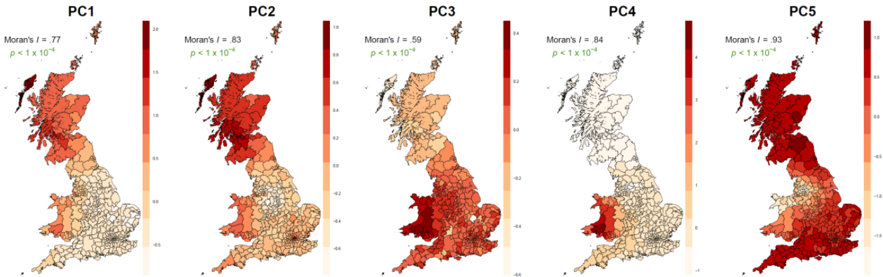
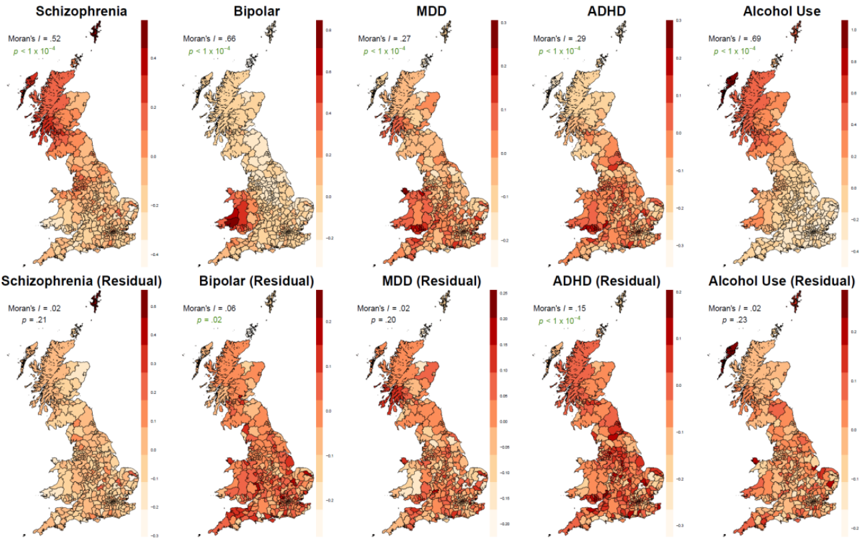
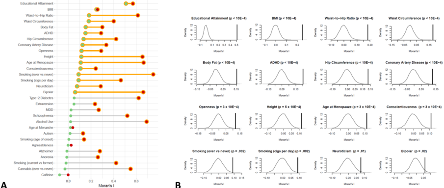
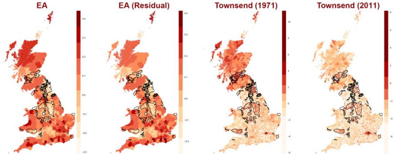
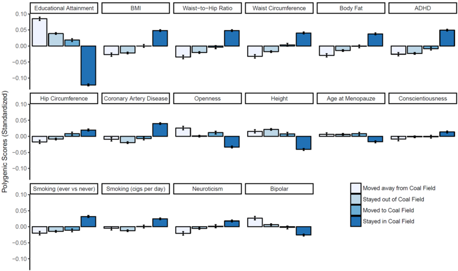
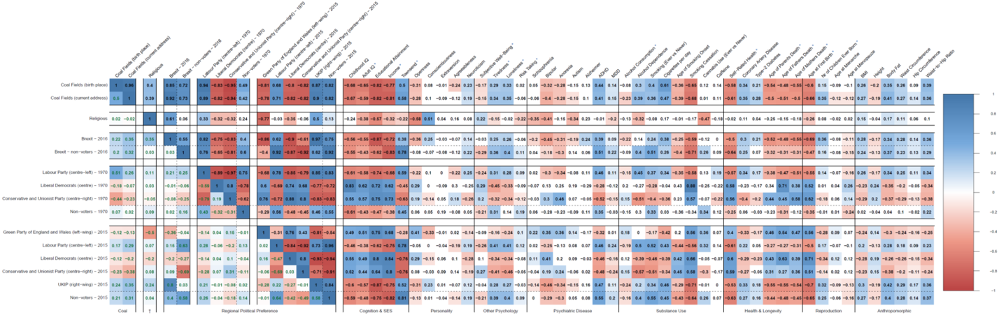
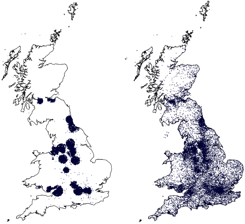
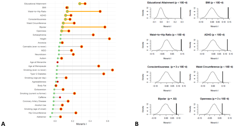
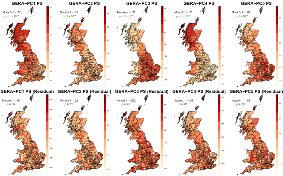
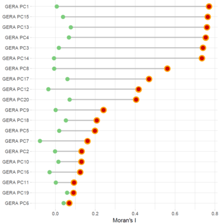
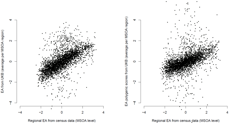
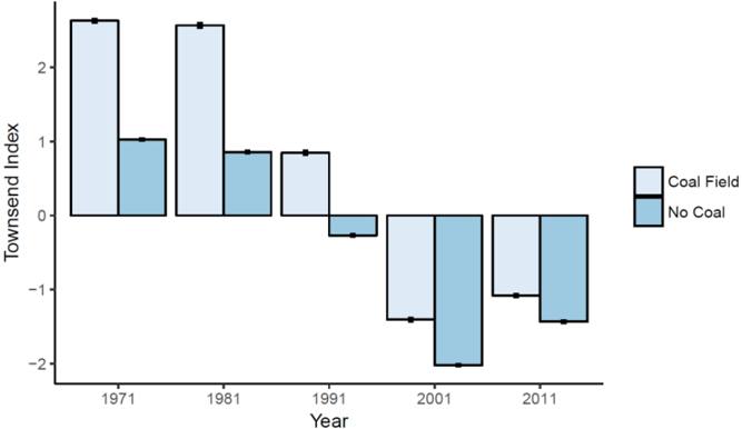
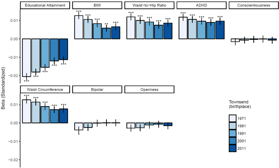
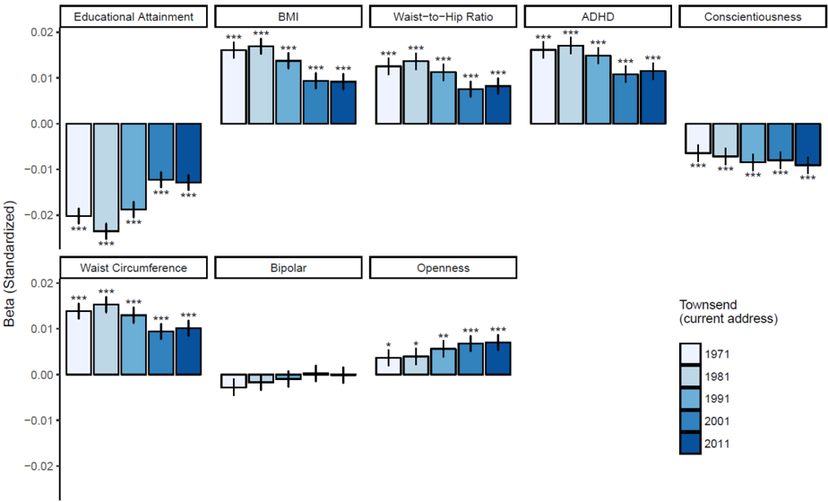
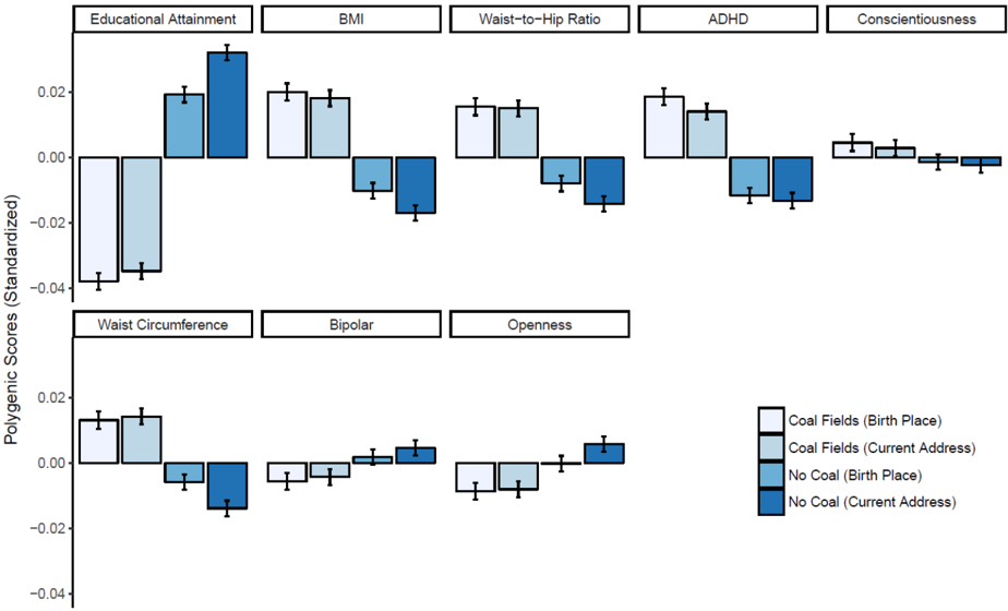
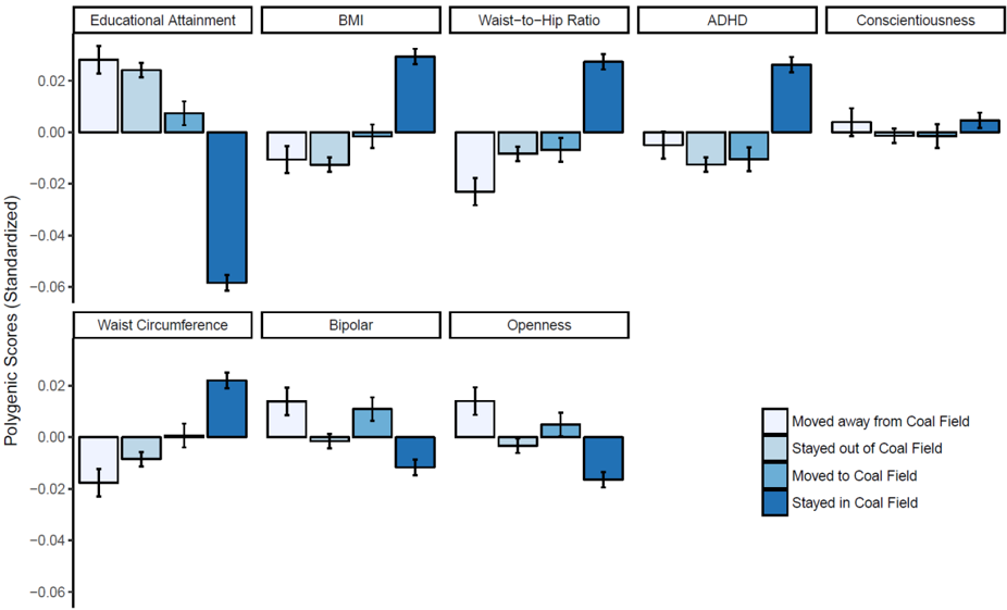
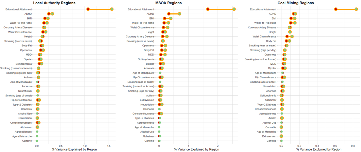
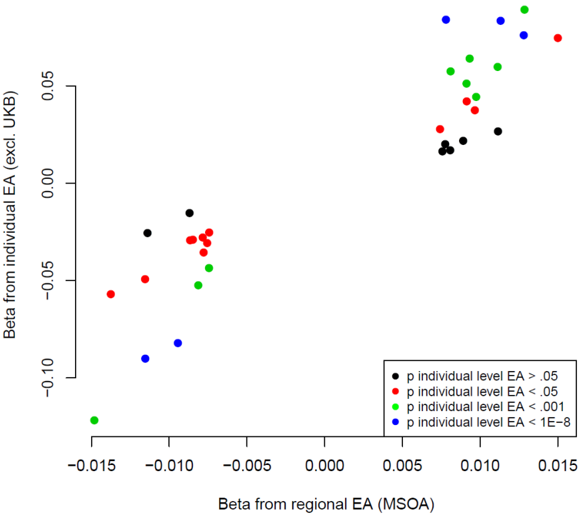
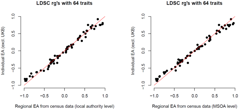
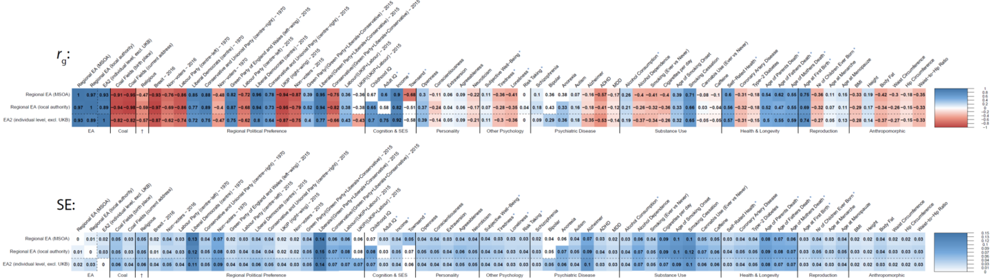
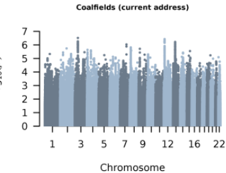
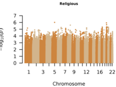
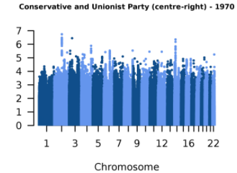
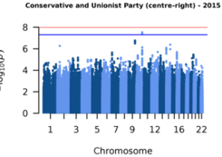
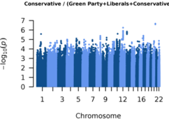
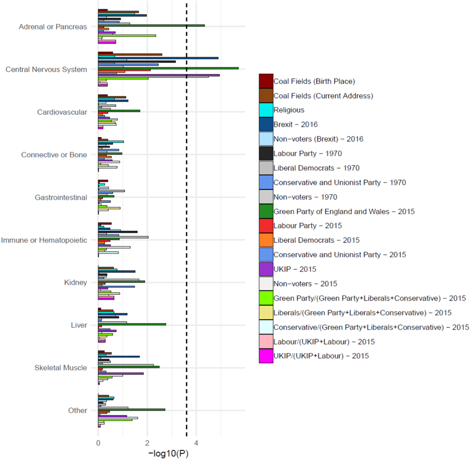
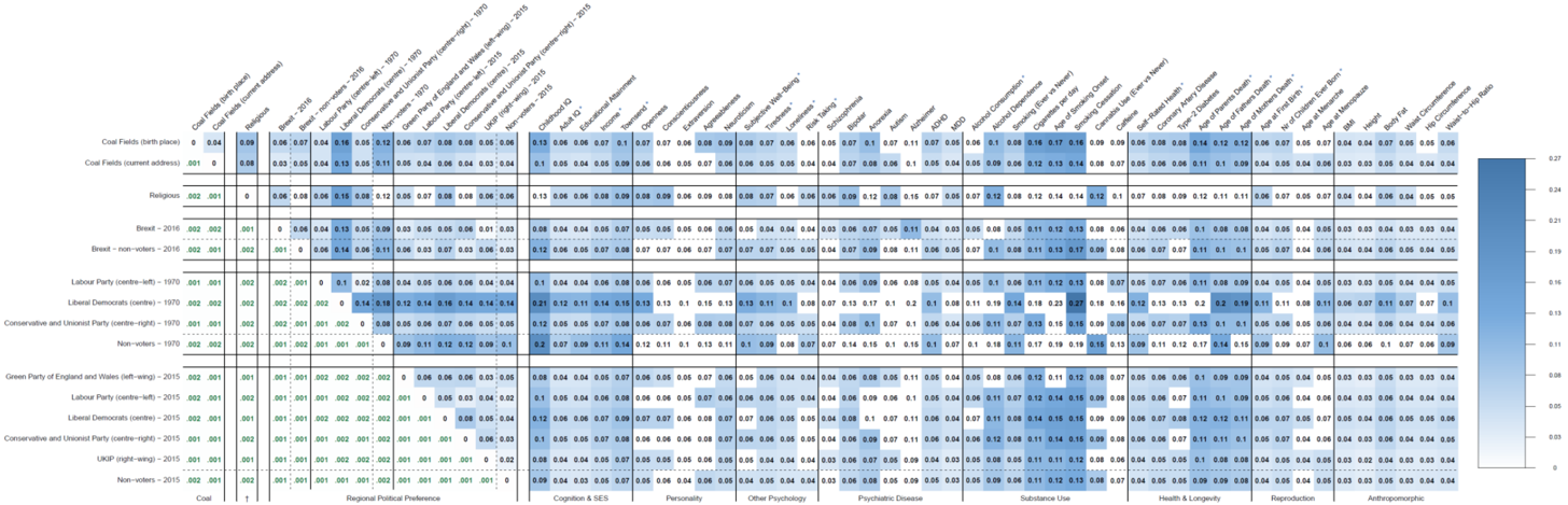
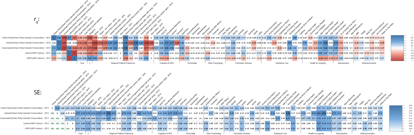
Human DNA polymorphisms vary across geographic regions, with the most commonly observed variation reflecting distant ancestry differences. Here we investigate the geographic clustering of common genetic variants that influence complex traits in a sample of ~450,000 individuals from Great Britain. Of 33 traits analysed, 21 showed significant geographic clustering at the genetic level after controlling for ancestry, probably reflecting migration driven by socioeconomic status (SES). Alleles associated with educational attainment (EA) showed the most clustering, with EA-decreasing alleles clustering in lower SES areas such as coal mining areas. Individuals who leave coal mining areas carry more EA-increasing alleles on average than those in the rest of Great Britain. The level of geographic clustering is correlated with genetic associations between complex traits and regional measures of SES, health and cultural outcomes. Our results are consistent with the hypothesis that social stratification leaves visible marks in geographic arrangements of common allele frequencies and gene-environment correlations.
Overview
The claims and statistics of this paper haven’t been checked yet.
Run the check — free, no account needed. It reads the open-access text and checks the sources it cites.
Integrity signals
Registry
Cites
Statistics
Figures
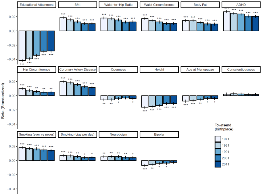
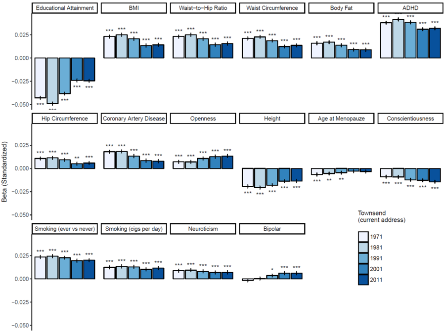
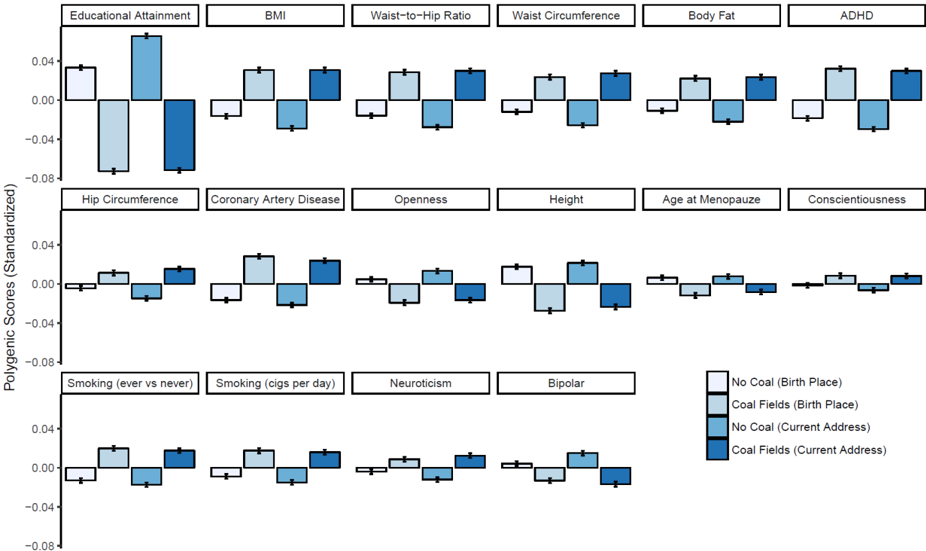
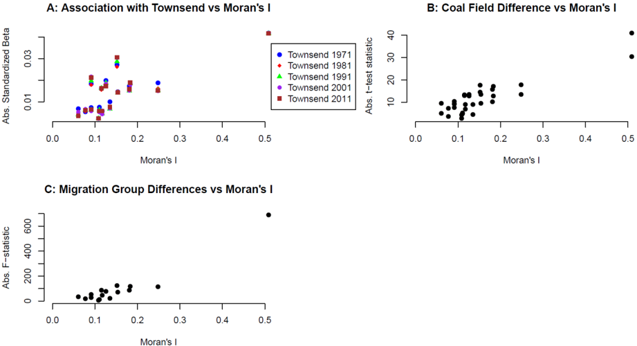
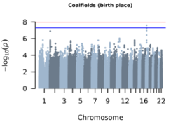
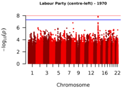
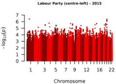
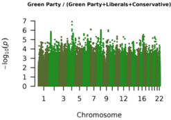
Verification
Claims the paper makes
The claims and statistics of this paper haven’t been checked yet.
Run the check — free, no account needed. It reads the open-access text and checks the sources it cites.
Claims other papers make about this one
Each is checked against this paper’s own text: does it say what the citing paper says it does?
The source backs part of the claim, not all of it — or backs it for a different population, condition or comparison.
In the citing paper
“This remainder is due to assortment on phenotypes correlated with the EA PGI other than EA, cognitive performance, and vocabulary—possibly including various personality traits42-44—and sources of social homogamy other than genetic ancestry captured by the top 40 PCs—possibly including geographic location at courtship age45,46, socioeconomic status, and social class47.”
From Polygenic prediction of educational attainment within and between families from genome-wide association analyses in 3 million individuals (2022) · cites this paper as [46]
Experimental — accuracy not yet measured
Self-check
Percentages, sums and reported differences re-computed from the paper’s own numbers.
The self-check needs the paper’s full text.
Citations
Cites
PLINK: a tool set for whole-genome association and population-based linkage analyses.
Purcell, S., Neale, B., Todd-Brown, K., Thomas, L., Ferreira, M. A. R., Bender, D., Maller, J., Sklar, P., de Bakker, P. I. W., Daly, M. J., et al. (2007) · The American Journal of Human Genetics · doi:10.1086/519795 · Cited by 34,089
A global reference for human genetic variation
The 1000 Genomes Project Consortium, authors, C., Auton, A., Abecasis, G. R., Steering committee, Altshuler, D. M., Durbin, R. M., Abecasis, G. R., Bentley, D. R., Chakravarti, A., et al. (2015) · Nature · doi:10.1038/nature15393 · Cited by 18,247
Sudlow, C., Gallacher, J., Allen, N., Beral, V., Burton, P., Danesh, J., Downey, P., Elliott, P., Green, J., Landray, M., et al. (2015) · PLOS Medicine · doi:10.1371/journal.pmed.1001779 · Cited by 12,728
Principal components analysis corrects for stratification in genome-wide association studies
Price, A. L., Patterson, N. J., Plenge, R. M., Weinblatt, M. E., Shadick, N. A., & Reich, D. (2006) · Nature Genetics · doi:10.1038/ng1847 · Cited by 10,248
A Computer Movie Simulating Urban Growth in the Detroit Region
Tobler, W. (1970) · Economic Geography · doi:10.2307/143141 · Cited by 10,095
The UK Biobank resource with deep phenotyping and genomic data
Bycroft, C., Freeman, C., Petkova, D., Band, G., Elliott, L. T., Sharp, K., Motyer, A., Vukcevic, D., Delaneau, O., O’Connell, J., et al. (2018) · Nature · doi:10.1038/s41586-018-0579-z · Cited by 8,876
NOTES ON CONTINUOUS STOCHASTIC PHENOMENA
MORAN, P. A. P. (1950) · Biometrika · doi:10.1093/biomet/37.1-2.17 · Cited by 8,622
GCTA: a tool for genome-wide complex trait analysis
Yang, J., Lee, S. H., Goddard, M. E., & Visscher, P. M. (2011) · The American Journal of Human Genetics · doi:10.1016/j.ajhg.2010.11.011 · Cited by 8,279
Self-citationBiological insights from 108 schizophrenia-associated genetic loci
Schizophrenia Working Group of the Psychiatric Genomics Consortium (2014) · Nature · doi:10.1038/nature13595 · Cited by 7,577
Davey Smith, G., & Ebrahim, S. (2003) · International Journal of Epidemiology · doi:10.1093/ije/dyg070 · Cited by 5,882
Research works printed but not linked: 1
- Townsend, P., Phillimore, P. & Beattie, A. Health and Deprivation: Inequality and the North (Routledge, 1988).
Cited by
Sorted by citations
Genome-wide association studies
Uffelmann, E., Huang, Q. Q., Munung, N. S., de Vries, J., Okada, Y., Martin, A. R., Martin, H. C., Lappalainen, T., & Posthuma, D. (2021) · Nature Reviews Methods Primers · doi:10.1038/s43586-021-00056-9 · Cited by 1,849
Mendelian Randomization: Concepts and Scope
Richmond, R. C., & Davey Smith, G. (2022) · Cold Spring Harbor Perspectives in Medicine · doi:10.1101/cshperspect.a040501 · Cited by 841
Okbay, A., Wu, Y., Wang, N., Jayashankar, H., Bennett, M., Nehzati, S. M., Sidorenko, J., Kweon, H., Goldman, G., Gjorgjieva, T., et al. (2022) · Nature Genetics · doi:10.1038/s41588-022-01016-z · Cited by 654
Self-citation15 years of GWAS discovery: Realizing the promise
Abdellaoui, A., Yengo, L., Verweij, K. J. H., & Visscher, P. M. (2023) · The American Journal of Human Genetics · doi:10.1016/j.ajhg.2022.12.011 · Cited by 570
Self-citationRichardson, T. G., Harrison, S., Hemani, G., & Davey Smith, G. (2019) · eLife · doi:10.7554/elife.43657 · Cited by 198
Using genetics for social science
Harden, K. P., & Koellinger, P. D. (2020) · Nature Human Behaviour · doi:10.1038/s41562-020-0862-5 · Cited by 180
Discovery and implications of polygenicity of common diseases
Visscher, P. M., Yengo, L., Cox, N. J., & Wray, N. R. (2021) · Science · doi:10.1126/science.abi8206 · Cited by 199
Self-citationGenome-wide analysis identifies molecular systems and 149 genetic loci associated with income
Hill, W. D., Davies, N. M., Ritchie, S. J., Skene, N., Bryois, J., Bell, S., Angelantonio, E. D., Roberts, D. J., Shen, X., Davies, G., et al. (2019) · Nature Communications · doi:10.1038/s41467-019-13585-5 · Cited by 186
Resource profile and user guide of the Polygenic Index Repository
Becker, J., Burik, C. A. P., Goldman, G., Wang, N., Jayashankar, H., Bennett, M., Belsky, D. W., Linnér, R. K., Ahlskog, R., Kleinman, A., et al. (2021) · Nature Human Behaviour · doi:10.1038/s41562-021-01119-3 · Cited by 179
Self-citationWithin family Mendelian randomization studies
Davies, N. M., Howe, L. J., Brumpton, B., Havdahl, A., Evans, D. M., & Davey Smith, G. (2019) · Human Molecular Genetics · doi:10.1093/hmg/ddz204 · Cited by 158
Gene–environment correlations across geographic regions affect genome-wide association studies
Abdellaoui, A., Dolan, C. V., Verweij, K. J. H., & Nivard, M. G. (2022) · Nature Genetics · doi:10.1038/s41588-022-01158-0 · Cited by 163
Self-citationSociology, Genetics, and the Coming of Age of Sociogenomics
Mills, M. C., & Tropf, F. C. (2020) · Annual Review of Sociology · doi:10.1146/annurev-soc-121919-054756 · Cited by 162
Demographic history mediates the effect of stratification on polygenic scores
Zaidi, A. A., & Mathieson, I. (2020) · eLife · doi:10.7554/elife.61548 · Cited by 122
Mendelian imputation of parental genotypes improves estimates of direct genetic effects
Young, A. I., Nehzati, S. M., Benonisdottir, S., Okbay, A., Jayashankar, H., Lee, C., Cesarini, D., Benjamin, D. J., Turley, P., & Kong, A. (2022) · Nature Genetics · doi:10.1038/s41588-022-01085-0 · Cited by 144
Hu, X., Zhao, J., Lin, Z., Wang, Y., Peng, H., Zhao, H., Wan, X., & Yang, C. (2022) · Proceedings of the National Academy of Sciences · doi:10.1073/pnas.2106858119 · Cited by 132
Gidziela, A., Ahmadzadeh, Y. I., Michelini, G., Allegrini, A. G., Agnew‐Blais, J. C., Lau, L. Y., Duret, M., Procopio, F., Daly, E., Ronald, A., et al. (2023) · Nature Human Behaviour · doi:10.1038/s41562-023-01530-y · Cited by 132
Sanderson, E., Richardson, T. G., Hemani, G., & Davey Smith, G. (2021) · International Journal of Epidemiology · doi:10.1093/ije/dyaa288 · Cited by 115
Intelligence, health and death
Deary, I. J., Hill, W. D., & Galé, C. R. (2021) · Nature Human Behaviour · doi:10.1038/s41562-021-01078-9 · Cited by 111
Dissecting polygenic signals from genome-wide association studies on human behaviour
Abdellaoui, A., & Verweij, K. J. H. (2021) · Nature Human Behaviour · doi:10.1038/s41562-021-01110-y · Cited by 104
Self-citationGreenstone, H., Wootton, R. E., Abdellaoui, A., Denys, D. A. J. P., Verweij, K. J. H., Munafo, M. R., & Treur, J. L. (2020) · Addiction · doi:10.1111/add.15142 · Cited by 99
Self-citationCultural evolution of genetic heritability
Uchiyama, R., Spicer, R., & Muthukrishna, M. (2021) · Behavioral and Brain Sciences · doi:10.1017/s0140525x21000893 · Cited by 103
The use of Mendelian randomisation to identify causal cancer risk factors: promise and limitations
Gala, H., & Tomlinson, I. P. M. (2020) · The Journal of Pathology · doi:10.1002/path.5421 · Cited by 86
Nivard, M. G., Belsky, D. W., Harden, K. P., Baier, T., Andreassen, O. A., Ystrøm, E., van Bergen, E., & Lyngstad, T. H. (2024) · Nature Human Behaviour · doi:10.1038/s41562-023-01796-2 · Cited by 65
Self-citationMarees, A. T., Smit, D. J. A., Abdellaoui, A., Nivard, M. G., van den Brink, W., Denys, D. A. J. P., Galama, T. J., Verweij, K. J. H., & Derks, E. M. (2021) · Nature Human Behaviour · doi:10.1038/s41562-021-01053-4 · Cited by 74
Self-citationCharacterizing the Genetic Overlap Between Psychiatric Disorders and Sleep-Related Phenotypes
O’Connell, K. S., Frei, O., Bahrami, S., Smeland, O. B., Bettella, F., Cheng, W., Chu, Y., Hindley, G., Lin, A., Shadrin, A. A., et al. (2021) · Biological Psychiatry · doi:10.1016/j.biopsych.2021.07.007 · Cited by 72
Ebert, T., Gebauer, J. E., Brenner, T., Bleidorn, W., Gosling, S. D., Potter, J., & Rentfrow, P. J. (2021) · Perspectives on Psychological Science · doi:10.1177/1745691621998326 · Cited by 88
Inferring Gene-by-Environment Interactions with a Bayesian Whole-Genome Regression Model
Kerin, M., & Marchini, J. (2020) · The American Journal of Human Genetics · doi:10.1016/j.ajhg.2020.08.009 · Cited by 65
Modeling assortative mating and genetic similarities between partners, siblings, and in-laws
Torvik, F. A., Eilertsen, E. M., Hannigan, L. J., Cheesman, R., Howe, L. J., Magnus, P. M., Reichborn‐Kjennerud, T., Andreassen, O. A., Njølstad, P. R., Havdahl, A., et al. (2022) · Nature Communications · doi:10.1038/s41467-022-28774-y · Cited by 65
Can education be personalised using pupils’ genetic data?
Morris, T., Davies, N. M., & Smith, G. D. (2020) · eLife · doi:10.7554/elife.49962 · Cited by 62
Mendelian randomization: the challenge of unobserved environmental confounds
Koellinger, P., & de Vlaming, R. (2019) · International Journal of Epidemiology · doi:10.1093/ije/dyz138 · Cited by 61
Polygenic Risk Scores Derived From Varying Definitions of Depression and Risk of Depression
Mitchell, B. L., Thorp, J. G., Wu, Y., Campos, A. I., Nyholt, D. R., Gordon, S. D., Whiteman, D. C., Olsen, C. M., Hickie, I. B., Martin, N. G., et al. (2021) · JAMA Psychiatry · doi:10.1001/jamapsychiatry.2021.1988 · Cited by 66
Self-citationHarrison, S., Davies, A. R., Dickson, M., Tyrrell, J., Green, M. J., Katikireddi, S. V., Campbell, D., Munafo, M. R., Dixon, P., Jones, H. E., et al. (2020) · International Journal of Epidemiology · doi:10.1093/ije/dyaa114 · Cited by 63
Hu, S., Ferreira, L. A. F., Shi, S., Hellenthal, G., Marchini, J., Lawson, D. J., & Myers, S. (2025) · Nature Genetics · doi:10.1038/s41588-024-02035-8 · Cited by 75
Timmers, P. R. H. J., Tiys, E., Sakaue, S., Akiyama, M., Kiiskinen, T., Zhou, W., Hwang, S., Yao, C., Biobank Japan Project, Kamatani, Y., et al. (2022) · Nature Aging · doi:10.1038/s43587-021-00159-8 · Cited by 59
Erola, J., Lehti, H., Baier, T., & Karhula, A. (2021) · European Sociological Review · doi:10.1093/esr/jcab026 · Cited by 57
Maxwell, J. M., Coleman, J. R. I., Breen, G. D., & Vassos, E. (2021) · JAMA Psychiatry · doi:10.1001/jamapsychiatry.2021.2983 · Cited by 54
Multivariable G-E interplay in the prediction of educational achievement
Allegrini, A. G., Karhunen, V., Coleman, J. R. I., Selzam, S., Rimfeld, K., von Stumm, S., Pingault, J., & Plomin, R. J. (2020) · PLoS Genetics · doi:10.1371/journal.pgen.1009153 · Cited by 54
Modeling environment through a general exposome factor in two independent adolescent cohorts
Moore, T. M., Visoki, E., Argabright, S. T., DiDomenico, G. E., Sotelo, I., Wortzel, J. D., Naeem, A., Gur, R. C., Gur, R. E., Warrier, V., et al. (2022) · Exposome · doi:10.1093/exposome/osac010 · Cited by 60
Association of Economic Status and Educational Attainment With Posttraumatic Stress Disorder
Polimanti, R. A., Ratanatharathorn, A. D., Maihofer, A. X., Choi, K. W., Stein, M. B., Morey, R. A., Logue, M. W., Nievergelt, C. M., Stein, D. J., Koenen, K. C., et al. (2019) · JAMA Network Open · doi:10.1001/jamanetworkopen.2019.3447 · Cited by 55
Phenotypic covariance across the entire spectrum of relatedness for 86 billion pairs of individuals
Kemper, K. E., Yengo, L., Zheng, Z., Abdellaoui, A., Keller, M. C., Goddard, M. E., Wray, N. R., Yang, J., & Visscher, P. M. (2021) · Nature Communications · doi:10.1038/s41467-021-21283-4 · Cited by 43
Self-citationA framework for research into continental ancestry groups of the UK Biobank
Constantinescu, A., Mitchell, R. E., Zheng, J., Bull, C. J., Timpson, N. J., Amulic, B., Vincent, E. E., & Hughes, D. A. (2022) · Human Genomics · doi:10.1186/s40246-022-00380-5 · Cited by 49
Genetic Risk for Smoking: Disentangling Interplay Between Genes and Socioeconomic Status
Pasman, J. A., Demange, P. A., Guloksuz, S., Willemsen, A. H. M., Abdellaoui, A., ten Have, M., Hottenga, J.-J., Boomsma, D. I., de Geus, E., Bartels, M., et al. (2022) · Behavior Genetics · doi:10.1007/s10519-021-10094-4 · Cited by 41
Self-citationNiarchou, M., Byrne, E. M., Trzaskowski, M., Sidorenko, J., Kemper, K. E., McGrath, J. J., O’Donovan, M. C., Owen, M. J., & Wray, N. R. (2020) · Translational Psychiatry · doi:10.1038/s41398-020-0688-y · Cited by 46
Self-citationCarvalho, C. M., Wendt, F. R., Maihofer, A. X., Stein, D. J., Stein, M. B., Sumner, J. A., Hemmings, S. M. J., Nievergelt, C. M., Koenen, K. C., Gelernter, J. E., et al. (2020) · Neuropsychopharmacology · doi:10.1038/s41386-020-0655-6 · Cited by 46
Polygenic Scores in Developmental Psychology: Invite Genetics In, Leave Biodeterminism Behind
Raffington, L., Mallard, T. T., & Harden, K. P. (2020) · Annual Review of Developmental Psychology · doi:10.1146/annurev-devpsych-051820-123945 · Cited by 44
The Potential Impact of Social Genomics on Wound Healing
Fayne, R. A., Borda, L. J., Egger, A. N., & Tomic‐Canic, M. (2019) · Advances in Wound Care · doi:10.1089/wound.2019.1095 · Cited by 48
Harrison, S., Davies, N. M., Howe, L. D., & Hughes, A. (2021) · Science Advances · doi:10.1126/sciadv.abf8257 · Cited by 44
Jelenkovic, A., Sund, R., Yokoyama, Y., Latvala, A., Sugawara, M., TANAKA, M., Matsumoto, S., Freitas, D. L., Maia, J. A. R., Knafo‐Noam, A., et al. (2020) · Scientific Reports · doi:10.1038/s41598-020-64883-8 · Cited by 44
Marchi, M., Alkema, A., Xia, C., Thio, C. H. L., Chen, L.-Y., Schalkwijk, W., Galeazzi, G. M., Ferrari, S., Pingani, L., Kweon, H., et al. (2024) · Nature Human Behaviour · doi:10.1038/s41562-024-01919-3 · Cited by 47
Multi-omic spatial effects on high-resolution AI-derived retinal thickness
Jackson, V. E., Wu, Y., Bonelli, R., Owen, J. P., Scott, L. W., Farashi, S., Kihara, Y., Gantner, M. L., Egan, C. A., Williams, K. M., et al. (2025) · Nature Communications · doi:10.1038/s41467-024-55635-7 · Cited by 35
Sariaslan, A., Mikkonen, J., Aaltonen, M., Hiilamo, H., Martikainen, P., & Fazel, S. (2021) · International Journal of Epidemiology · doi:10.1093/ije/dyab099 · Cited by 48
Dutch population structure across space, time and GWAS design
Byrne, R. P., van Rheenen, W., van den Berg, L. H., Veldink, J. H., & McLaughlin, R. L. (2020) · Nature Communications · doi:10.1038/s41467-020-18418-4 · Cited by 39
Genetic predictors of educational attainment and intelligence test performance predict voter turnout
Aarøe, L., Appadurai, V., Hansen, K. M., Schork, A. J., Werge, T. M., Mors, O. N., Børglum, A. D., HOUGAARD, D. M., Nordentoft, M., Mortensen, P. B., et al. (2020) · Nature Human Behaviour · doi:10.1038/s41562-020-00952-2 · Cited by 37
The importance of family-based sampling for biobanks
Davies, N. M., Hemani, G., Neiderhiser, J. M., Martin, H. C., Mills, M. C., Visscher, P. M., Yengo, L., Young, A. I., & Keller, M. C. (2024) · Nature · doi:10.1038/s41586-024-07721-5 · Cited by 34
Self-citationSubstance use: Interplay between polygenic risk and neighborhood environment
Pasman, J. A., Verweij, K. J. H., Abdellaoui, A., Hottenga, J., Fedko, I. O., Willemsen, G. A. H. M., Boomsma, D. I., & Vink, J. M. (2020) · Drug and Alcohol Dependence · doi:10.1016/j.drugalcdep.2020.107948 · Cited by 34
Self-citationThe CADM2 Gene and Behavior: A Phenome-Wide Scan in UK-Biobank
Pasman, J. A., Chen, Z., Smit, D. J. A., Vink, J. M., van den Oever, M. C., Pattij, T., Vries, T. J. D., Abdellaoui, A., & Verweij, K. J. H. (2022) · Behavior Genetics · doi:10.1007/s10519-022-10109-8 · Cited by 30
Self-citationConcerns about the use of polygenic embryo screening for psychiatric and cognitive traits
Lencz, T., Sabatello, M., Docherty, A. R., Peterson, R. E., Soda, T., Austin, J., Bierut, L. J., Crepaz‐Keay, D., Curtis, D., Degenhardt, F., et al. (2022) · The Lancet Psychiatry · doi:10.1016/s2215-0366(22)00157-2 · Cited by 39
The gene-based hack that is revolutionizing epidemiology
Adam, D. (2019) · Nature · doi:10.1038/d41586-019-03754-3 · Cited by 31
A model and test for coordinated polygenic epistasis in complex traits
Sheppard, B. K., Rappoport, N., Loh, P., Sanders, S., Zaitlen, N., & Dahl, A. W. (2021) · Proceedings of the National Academy of Sciences · doi:10.1073/pnas.1922305118 · Cited by 31
Rare genetic variants explain missing heritability in smoking
Jang, S.-K., Evans, L. M., Fialkowski, A., Arnett, D. K., Ashley‐Koch, A. E., Barnes, K. C., Becker, D. M., Bis, J. C., Blangero, J., Bleecker, E. R., et al. (2022) · Nature Human Behaviour · doi:10.1038/s41562-022-01408-5 · Cited by 29
From Genome-Wide to Environment-Wide: Capturing the Environome
von Stumm, S., & d’Apice, K. (2021) · Perspectives on Psychological Science · doi:10.1177/1745691620979803 · Cited by 32
Smit, D. J. A., Andreassen, O. A., Boomsma, D. I., Burwell, S. J., Chorlian, D. B., de Geus, E. J. C., Elvsåshagen, T., Gordon, R. L., Harper, J., Hegerl, U., et al. (2021) · Brain and Behavior · doi:10.1002/brb3.2188 · Cited by 34
The promise and peril of the new science of social genomics
Adam, D. (2019) · Nature · doi:10.1038/d41586-019-03171-6 · Cited by 29
Entrepreneurship in the Long-Run: Empirical Evidence and Historical Mechanisms
Fritsch, M. J., & Wyrwich, M. (2023) · Foundations and Trends® in Entrepreneurship · doi:10.1561/0300000100 · Cited by 34
Cai, M., Wang, Z., Xiao, J., Hu, X., Chen, G., & Yang, C. (2023) · Nature Communications · doi:10.1038/s41467-023-42614-7 · Cited by 26
Heritable polygenic editing: the next frontier in genomic medicine?
Visscher, P. M., Gyngell, C., Yengo, L., & Savulescu, J. (2025) · Nature · doi:10.1038/s41586-024-08300-4 · Cited by 33
Self-citationXPXP: improving polygenic prediction by cross-population and cross-phenotype analysis
Xiao, J., Cai, M., Hu, X., Wan, X., Chen, G., & Yang, C. (2022) · Bioinformatics · doi:10.1093/bioinformatics/btac029 · Cited by 24
Quantitative Human Paleogenetics: What can Ancient DNA Tell us About Complex Trait Evolution?
Irving-Pease, E. K., Muktupavela, R., Dannemann, M., & Racimo, F. (2021) · Frontiers in Genetics · doi:10.3389/fgene.2021.703541 · Cited by 27
Minică, C. C., Boomsma, D. I., Dolan, C. V., de Geus, E., & Neale, M. C. (2020) · International Journal of Epidemiology · doi:10.1093/ije/dyaa013 · Cited by 23
Liu, S., Smit, D. J. A., Abdellaoui, A., van Wingen, G. A., & Verweij, K. J. H. (2022) · Biological Psychiatry Cognitive Neuroscience and Neuroimaging · doi:10.1016/j.bpsc.2022.08.003 · Cited by 25
Self-citationCausal Inference Methods to Integrate Omics and Complex TraitsPreprint
Porcu, E., Sjaarda, J., Lepik, K., Carmeli, C., Darrous, L., Sulc, J., Mounier, N., & Kutalik, Z. (2020) · Cold Spring Harbor Perspectives in Medicine · doi:10.1101/cshperspect.a040493 · Cited by 23
Why do we pick similar mates, or do we?
Versluys, T. M. M., Mas-Sandoval, À., Flintham, E. O., & Savolainen, V. (2021) · Biology Letters · doi:10.1098/rsbl.2021.0463 · Cited by 22
A polygenic score for educational attainment partially predicts voter turnout
Dawes, C. T., Okbay, A., Oskarsson, S., & Rustichini, A. (2021) · Proceedings of the National Academy of Sciences · doi:10.1073/pnas.2022715118 · Cited by 23
A Systematic Framework for Assessing the Clinical Impact of Polygenic Risk ScoresPreprint
Kulm, S., Marderstein, A. R., Mezey, J. G., & Elemento, O. (2020) · SSRN Electronic Journal · doi:10.1101/2020.04.06.20055574 · Cited by 25
An evolutionary perspective on complex neuropsychiatric disease
McClellan, J., Zoghbi, A. W., Buxbaum, J. D., Cappi, C., Crowley, J. J., Flint, J., Grice, D. E., Gülsüner, S., Iyegbe, C. O., Jain, S., et al. (2023) · Neuron · doi:10.1016/j.neuron.2023.10.037 · Cited by 25
Expanding the environmental scope: an environment-wide association study for mental well-being
van de Weijer, M. P., Baselmans, B. M. L., Hottenga, J., Dolan, C. V., Willemsen, G. A. H. M., & Bartels, M. (2021) · Journal of Exposure Science & Environmental Epidemiology · doi:10.1038/s41370-021-00346-0 · Cited by 25
Judd, N., Sauce, B., & Klingberg, T. (2022) · npj Science of Learning · doi:10.1038/s41539-022-00148-5 · Cited by 27
Barcellos, S., Carvalho, L., & Turley, P. (2021) · National Bureau of Economic Research · doi:10.3386/w28750 · Cited by 24
Virtues as protective factors for adolescent mental health
McLoughlin, S., & Kristjansson, K. R. (2024) · Journal of Research on Adolescence · doi:10.1111/jora.13004 · Cited by 34
Socio-economic status is a social construct with heritable components and genetic consequences
Abdellaoui, A., Martin, H. C., Kolk, M., Rutherford, A. D., Muthukrishna, M., Tropf, F. C., Mills, M. C., Zietsch, B. P., Verweij, K. J. H., & Visscher, P. M. (2025) · Nature Human Behaviour · doi:10.1038/s41562-025-02150-4 · Cited by 39
Self-citationSmit, D. J. A., Bakker, M., Abdellaoui, A., Hoetink, A. E., Vulink, N. C. C., & Denys, D. A. J. P. (2023) · Frontiers in Neuroscience · doi:10.3389/fnins.2022.971752 · Cited by 25
Self-citationNivard, M. G., Belsky, D. W., Harden, K. P., Baier, T., Andreassen, O. A., Ystrøm, E., van Bergen, E., & Lyngstad, T. H. (2022) · doi:10.31234/osf.io/bhpm5 · Cited by 20
Self-citationSocial-Science Genomics: Progress, Challenges, and Future Directions
Benjamin, D., Cesarini, D., Turley, P., & Young, A. S. (2024) · doi:10.3386/w32404 · Cited by 20
Richardson, T. G., Mykkänen, J., Pahkala, K., Ala‐Korpela, M., Bell, J. A., Taylor, K., Viikari, J. S. A., Lehtimäki, T. J., Raitakari, O. T., & Smith, G. D. (2020) · medRxiv · doi:10.1101/2020.08.25.20181412 · Cited by 19
Pelt, D. H. M., Habets, P. C., Vinkers, C. H., Ligthart, L., van Beijsterveldt, C. E. M., Pool, R., & Bartels, M. (2024) · Nature Mental Health · doi:10.1038/s44220-024-00294-2 · Cited by 19
Gene-environment interplay in early life cognitive development
von Stumm, S., Kandaswamy, R., & Maxwell, J. M. (2023) · Intelligence · doi:10.1016/j.intell.2023.101748 · Cited by 20
Human Capital Mediates Natural Selection in Contemporary Humans
Hugh-Jones, D., & Abdellaoui, A. (2022) · Behavior Genetics · doi:10.1007/s10519-022-10107-w · Cited by 20
Self-citationLeveraging the local genetic structure for trans-ancestry association mapping
Xiao, J., Cai, M., Yu, X., Hu, X., Chen, G., Wan, X., & Yang, C. (2022) · The American Journal of Human Genetics · doi:10.1016/j.ajhg.2022.05.013 · Cited by 15
Jawinski, P., Forstbach, H., Kirsten, H., Beyer, F., Villringer, A., Witte, A. V., Scholz, M. R., Ripke, S., & Markett, S. A. (2025) · Nature Aging · doi:10.1038/s43587-025-00962-7 · Cited by 18
Personalized genealogical history of UK individuals inferred from biobank-scale IBD segments
Naseri, A., Tang, K., Geng, X., Shi, J., Zhang, J., Shakya, P., Liu, X., Zhang, S., & Zhi, D. (2021) · BMC Biology · doi:10.1186/s12915-021-00964-y · Cited by 15
Partner choice, confounding and trait convergence all contribute to phenotypic partner similarity
Sjaarda, J., & Kutalik, Z. (2023) · Nature Human Behaviour · doi:10.1038/s41562-022-01500-w · Cited by 16
Principal and independent genomic components of brain structure and function
Oblong, L. M., Soheili‐Nezhad, S., Trevisan, N., Shi, Y., Beckmann, C. F., & Sprooten, E. (2024) · Genes Brain & Behavior · doi:10.1111/gbb.12876 · Cited by 13
Topological stratification of continuous genetic variation in large biobanks
Diaz-Papkovich, A., Zabad, S., Snell, H., Ben-Eghan, C., Anderson-Trocmé, L., Femerling, G., Nathan, V., Patel, J., & Gravel, S. (2026) · PLoS Genetics · doi:10.1371/journal.pgen.1012068 · Cited by 15
McLoughlin, S., Tyndall, I. T., Pereira, A., & Mulhern, T. (2020) · Journal of Cognitive Enhancement · doi:10.1007/s41465-020-00187-z · Cited by 18
Multilevel Twin Models: Geographical Region as a Third Level Variable
Tamimy, Z., Kevenaar, S. T., Hottenga, J., Hunter, M. D., de Zeeuw, E. L., Neale, M. C., van Beijsterveldt, C. E. M., Dolan, C. V., van Bergen, E., & Boomsma, D. I. (2021) · Behavior Genetics · doi:10.1007/s10519-021-10047-x · Cited by 15
Moving back to the future of big data-driven research: reflecting on the social in genomics
Goisauf, M., Akyüz, K., & Martin, G. M. (2020) · Humanities and Social Sciences Communications · doi:10.1057/s41599-020-00544-5 · Cited by 19
Hu, S.-L., Ferreira, L. A. F., Shi, S., Hellenthal, G., Marchini, J., Lawson, D., & Myers, S. (2023) · bioRxiv · doi:10.1101/2023.08.08.552281 · Cited by 18
Understanding genetic variants in context
Sinnott-Armstrong, N., Fields, S., Roth, F. P., Starita, L. M., Trapnell, C., Villén, J., Fowler, D. M., & Queitsch, C. (2024) · eLife · doi:10.7554/elife.88231 · Cited by 14
Testing for differences in polygenic scores in the presence of confounding
Blanc, J., & Berg, J. J. (2025) · Genetics · doi:10.1093/genetics/iyaf071 · Cited by 15
The relationship between chronotype and intelligence: the importance of work timing
Ujma, P. P., Baudson, T. G., Bódizs, R., & Dresler, M. (2020) · Scientific Reports · doi:10.1038/s41598-020-62917-9 · Cited by 13
Metadata
- Authors
- Abdellaoui, A., Hugh-Jones, D., Yengo, L., Kemper, K. E., Nivard, M. G., Veul, L., Holtz, Y., Zietsch, B. P., Frayling, T. M., Wray, N. R., Yang, J., Verweij, K. J. H., & Visscher, P. M.
- Affiliations
- Amsterdam University Medical Centers (NL)
- University of East Anglia (GB)
- The University of Queensland (AU)
- Vrije Universiteit Amsterdam (NL)
- University of Exeter (GB)
- Corresponding author
- Abdellaoui, Abdel
- Visscher, Peter M.
- ORCID
- Venue
- Nature Human Behaviour
- Published
- 2019-10-21
- Volume
- 3
- Issue
- 12
- Pages
- 1332-1342
- ISSN
- 2397-3374 (ISSN-L)
- OpenAlex
- W2980548847
- Cited by
- 261
- References
- 100
- Citations by year
- 2026: 18 · 2025: 27 · 2024: 34 · 2023: 34 · 2022: 42 · 2021: 41 · 2020: 49 · 2019: 14
- FWCI
- 22.15
- Type
- journal article
- Language
- en
- Open access
- green
- doi.org
- Licence
- Locations
- Nature Human Behaviour (publishedVersion)
- bioRxiv (Cold Spring Harbor Laboratory) (acceptedVersion, cc-by-nc-nd)
- PubMed (publishedVersion)
- Pure Amsterdam UMC (publishedVersion, other-oa)
- VU Research Portal (publishedVersion, other-oa)
- Data Archiving and Networked Services (DANS) (submittedVersion, other-oa)
- Data Archiving and Networked Services (DANS) (submittedVersion)
- RePEc: Research Papers in Economics (submittedVersion)
- Royal Devon and Exeter Research Repository (Royal Devon and Exeter) (submittedVersion)
- UEA Digital Repository (University of East Anglia) (submittedVersion)
- Funders
- Ellison Medical Foundation
- Robert Wood Johnson Foundation
- Wayne and Gladys Valley Foundation
- Kaiser Permanente
- Wellcome Trust
- Scottish Government
- Llywodraeth Cymru
- Stichting Volksbond Rotterdam
- British Heart Foundation
- Diabetes UK
- ZonMw (849200011, 531003014)
- Northwest Regional Development Agency
- National Institutes of Health
- Medical Research Council (1107258, 1113400, 1078037, 1078901)
- Australian Research Council (FT160100298, 1113400)
- National Health and Medical Research Council (1113400, 1078901, 1056929, 1107258, 1078037, 1048853)
- National Institute on Aging (RC2AG036607)
- Topics
- Life Sciences › Biochemistry, Genetics and Molecular Biology › Genetics › Genetic Associations and Epidemiology
- Life Sciences › Biochemistry, Genetics and Molecular Biology › Genetics › Forensic and Genetic Research
- Social Sciences › Sociology and Political Science › Intergenerational and Educational Inequality Studies
- Keywords
- social stratification, educational attainment, socioeconomic status, gene-environment correlation, migration, coal mining areas, polygenic risk score, complex traits, regional health disparities, Great Britain
- MeSH terms
- Adipose Tissue, Alleles, Body Height, Educational Status, Emigration and Immigration, United Kingdom, Health Status, Humans, Phenotype, Social Class, Body Mass Index, Cluster Analysis, Multifactorial Inheritance, Polymorphism, Single Nucleotide, White People, Geographic Mapping
About these checks
Registry, retraction, Cites and statistics results are computed, not judged, with one exception: a printed reference that no index lists is read once by a model before it counts as a citation error. Claims are extracted by a model and kept only when their quote appears verbatim in the text; each cited source is then checked, with a model’s help, for whether it says what the claim relies on. Those verdicts can be wrong — read the claim’s quote and the cited source before relying on one.
Statistics and arithmetic are recomputed, not judged.
Confidence bands are shown only for fields calibrated on our annotated test set. None is calibrated yet, so no band is shown.
What counts as a claim ›How we measure confidence ›How we check this ›
Are you an author, or do you see a problem with this page? Request a review
