

The DOI matches its Crossref record; 21 of the 21 references it cites were found in a registry or an index.
Elevated genetic risk for multiple sclerosis emerged in steppe pastoralist populations
Published version of a preprint
Abstract
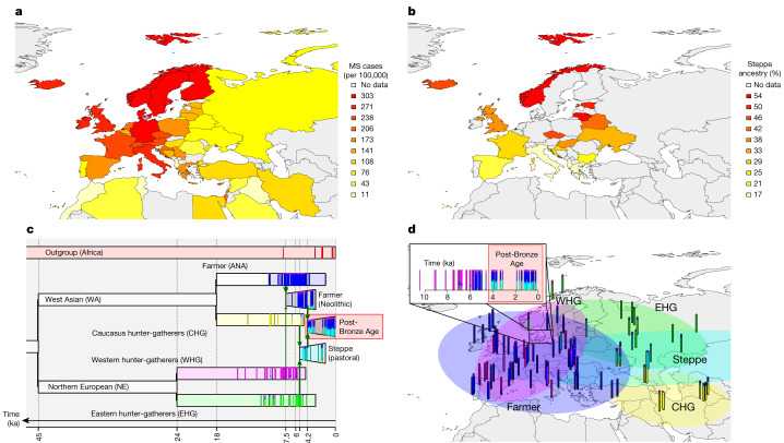
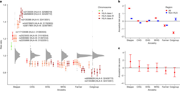
Multiple sclerosis (MS) is a neuro-inflammatory and neurodegenerative disease that is most prevalent in Northern Europe. Although it is known that inherited risk for MS is located within or in close proximity to immune-related genes, it is unknown when, where and how this genetic risk originated 1 . Here, by using a large ancient genome dataset from the Mesolithic period to the Bronze Age 2 , along with new Medieval and post-Medieval genomes, we show that the genetic risk for MS rose among pastoralists from the Pontic steppe and was brought into Europe by the Yamnaya-related migration approximately 5,000 years ago. We further show that these MS-associated immunogenetic variants underwent positive selection both within the steppe population and later in Europe, probably driven by pathogenic challenges coinciding with changes in diet, lifestyle and population density. This study highlights the critical importance of the Neolithic period and Bronze Age as determinants of modern immune responses and their subsequent effect on the risk of developing MS in a changing environment.
Overview
The claims and statistics of this paper haven’t been checked yet.
Run the check — free, no account needed. It reads the open-access text and checks the sources it cites.
Integrity signals
Registry
Cites
Statistics
Figures
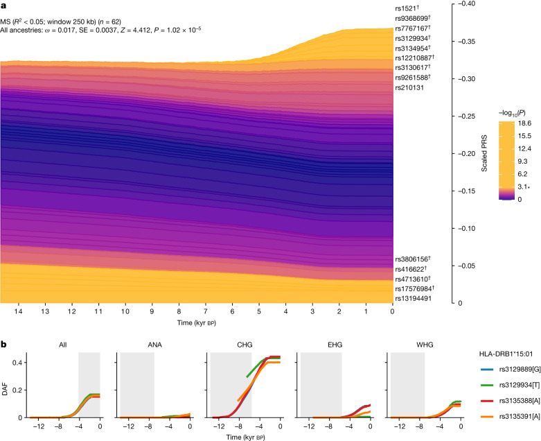
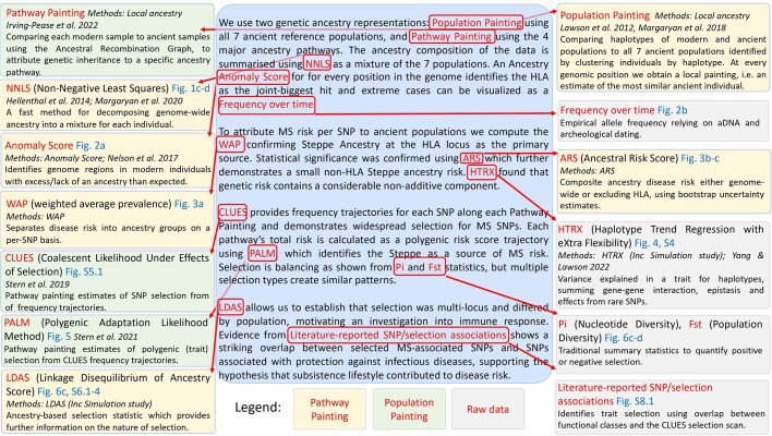
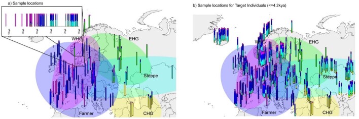
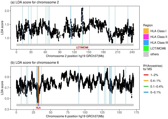
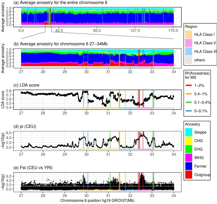
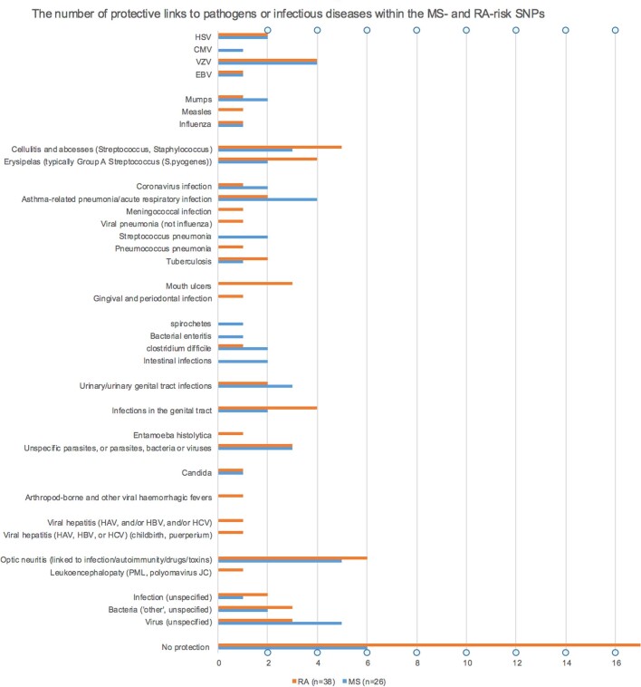
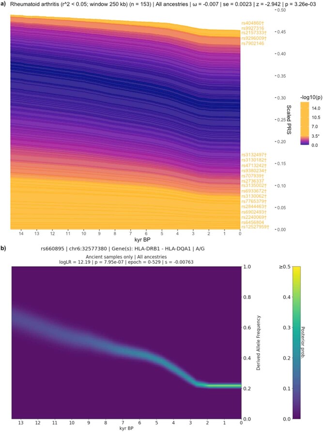
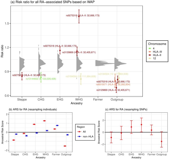
Verification
Claims the paper makes
The claims and statistics of this paper haven’t been checked yet.
Run the check — free, no account needed. It reads the open-access text and checks the sources it cites.
Claims other papers make about this one
Each is checked against this paper’s own text: does it say what the citing paper says it does?
The cited source says what the claim attributes to it.
In the citing paper
“First, modern disease risk may, in part, reflect ancient adaptive variation expressed in contemporary environments76.”
From Genetic trade-offs in fertility and longevity explain the maintenance of disease-associated alleles in humans (2026) · cites this paper as [76]
Self-check
Percentages, sums and reported differences re-computed from the paper’s own numbers.
The self-check needs the paper’s full text.
Citations
Cites
A global reference for human genetic variation
The 1000 Genomes Project Consortium, authors, C., Auton, A., Abecasis, G. R., Steering committee, Altshuler, D. M., Durbin, R. M., Abecasis, G. R., Bentley, D. R., Chakravarti, A., et al. (2015) · Nature · doi:10.1038/nature15393 · Cited by 18,247
Second-generation PLINK: rising to the challenge of larger and richer datasets
Chang, C. C., Chow, C. C., Tellier, L. C., Vattikuti, S., Purcell, S. M., & Lee, J. J. (2015) · Gigascience · doi:10.1186/s13742-015-0047-8 · Cited by 12,709
Feigin, V. L., Nichols, E., Alam, T., Bannick, M. S., Beghi, E., Blake, N., Culpepper, W. J., Dorsey, E. R., Elbaz, A., Ellenbogen, R. G., et al. (2019) · The Lancet Neurology · doi:10.1016/s1474-4422(18)30499-x · Cited by 5,644 · cited 3×
“…have inadvertently driven an increase in genetic risk for MS. Today, with increasing prevalence of MS cases observed over the last five decades 46,47 , we again observe a striking correlation with changes in our environment, including lifestyle choices and improved hygiene, which no longer…”
BackgroundFinnGen provides genetic insights from a well-phenotyped isolated population
Kurki, M. I., Karjalainen, J., Palta, P., Sipilä, T. P., Kristiansson, K., Donner, K. M., Reeve, M. P., Laivuori, H., Aavikko, M., Kaunisto, M. A., et al. (2023) · Nature · doi:10.1038/s41586-022-05473-8 · Cited by 4,233
ANGSD: Analysis of Next Generation Sequencing Data
Korneliussen, T. S., Albrechtsen, A., & Nielsen, R. (2014) · BMC Bioinformatics · doi:10.1186/s12859-014-0356-4 · Cited by 2,982
Self-citationAncient Admixture in Human History
Patterson, N., Moorjani, P., Luo, Y., Mallick, S., Rohland, N., Zhan, Y., Genschoreck, T., Webster, T., & Reich, D. (2012) · Genetics · doi:10.1534/genetics.112.145037 · Cited by 2,848
Bjornevik, K., Cortese, M., Healy, B. C., Kuhle, J., Mina, M. J., Leng, Y., Elledge, S. J., Niebuhr, D. W., Scher, A. I., Munger, K. L., et al. (2022) · Science · doi:10.1126/science.abj8222 · Cited by 2,049 · cited 22×
“A more detailed description of DNA extraction and library preparation can be found in Supplementary Note 1.”
BackgroundMethodInfluentialMassive migration from the steppe was a source for Indo-European languages in Europe
Haak, W., Lazaridis, I., Patterson, N., Rohland, N., Mallick, S., Llamas, B., Brandt, G., Nordenfelt, S., Harney, E., Stewardson, K., et al. (2015) · Nature · doi:10.1038/nature14317 · Cited by 1,940
mapDamage2.0: fast approximate Bayesian estimates of ancient DNA damage parameters
Jónsson, H., Ginolhac, A., Schubert, M., Johnson, P. L. F., & Orlando, L. (2013) · Bioinformatics · doi:10.1093/bioinformatics/btt193 · Cited by 1,669
Linkage disequilibrium--understanding the evolutionary past and mapping the medical future.
Slatkin, M. (2008) · Nature Reviews Genetics · doi:10.1038/nrg2361 · Cited by 1,614
Population genomics of Bronze Age Eurasia
Allentoft, M. E., Sikora, M., Sjögren, K.-G., Rasmussen, S., Rasmussen, M., Stenderup, J., Damgaard, P. B., Schroeder, H., Ahlström, T., Vinner, L., et al. (2015) · Nature · doi:10.1038/nature14507 · Cited by 1,550
Self-citationMultiple sclerosis genomic map implicates peripheral immune cells and microglia in susceptibility
International Multiple Sclerosis Genetics Consortium, Patsopoulos, N. A., Baranzini, S. E., Santaniello, A., Shoostari, P., Cotsapas, C., Wong, G., Beecham, A. H., James, T., Replogle, J., et al. (2019) · Science · doi:10.1126/science.aav7188 · Cited by 1,471
Inference of Population Structure using Dense Haplotype Data
Lawson, D. J., Hellenthal, G., Myers, S., & Falush, D. (2012) · PLoS Genetics · doi:10.1371/journal.pgen.1002453 · Cited by 1,188
Self-citationA Revised Timescale for Human Evolution Based on Ancient Mitochondrial Genomes
Fu, Q., Mittnik, A., Johnson, P. L. F., Bos, K., Lari, M., Bollongino, R., Sun, C., Giemsch, L., Schmitz, R., Burger, J., et al. (2013) · Current Biology · doi:10.1016/j.cub.2013.02.044 · Cited by 709
The Origins of Lactase Persistence in Europe
Itan, Y., Powell, A., Beaumont, M. A., Burger, J., & Thomas, M. G. (2009) · PLoS Computational Biology · doi:10.1371/journal.pcbi.1000491 · Cited by 569 · cited 1×
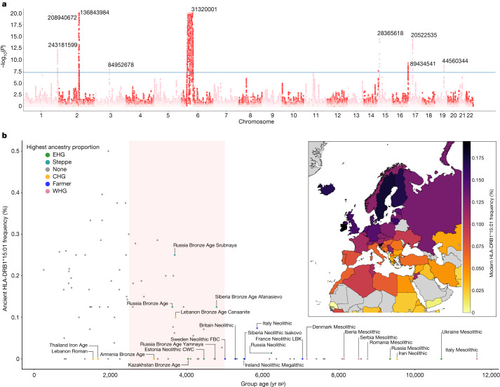
“2a): the LCT / MCM6 region on chromosome 2, which is well established as regulating lactase persistence 11,12 , and the HLA region on chromosome 6.”
BackgroundA population genetic signal of polygenic adaptation
Berg, J. J., & Coop, G. (2014) · PLoS Genetics · doi:10.1371/journal.pgen.1004412 · Cited by 487
Upper Palaeolithic genomes reveal deep roots of modern Eurasians
Jones, E. R., Gonzalez-Fortes, G., Connell, S., Siska, V., Eriksson, A., Martiniano, R., McLaughlin, R. L., Gallego Llorente, M., Cassidy, L. M., Gamba, C., et al. (2015) · Nature Communications · doi:10.1038/ncomms9912 · Cited by 417
The immunology of multiple sclerosis
Attfield, K. E., Jensen, L. T., Kaufmann, M., Friese, M. A., & Fugger, L. (2022) · Nature Reviews Immunology · doi:10.1038/s41577-022-00718-z · Cited by 380
Self-citationEstimating genetic kin relationships in prehistoric populations
Monroy Kuhn, J. M., Jakobsson, M., & Günther, T. (2018) · PLOS ONE · doi:10.1371/journal.pone.0195491 · Cited by 330
Comabella, M., Craig, D. W., Camiña-Tato, M., Morcillo, C., Lopez, C., Navarro, A., Rio, J., BiomarkerMS Study Group, Montalban, X., & Martin, R. (2008) · PLoS ONE · doi:10.1371/journal.pone.0003490 · Cited by 105
Genome‐wide association studies of multiple sclerosis
Cotsapas, C., & Mitrovic, M. (2018) · Clinical & Translational Immunology · doi:10.1002/cti2.1018 · Cited by 89
Research works printed but not linked: 62
- Allentoft, M. E. et al. Population genomics of post-glacial western Eurasia. Nature https://doi.org/10.1038/s41586-023-06865-0 (2024). · DOI
- Walton, C. et al. Rising prevalence of multiple sclerosis worldwide: insights from the Atlas of MS, third edition. Mult. Scler. J. 26, 1816–1821 (2020). · DOI
- Lanz, T. V. et al. Clonally expanded B cells in multiple sclerosis bind EBV EBNA1 and GlialCAM. Nature 603, 321–327 (2022). · DOI · Paper page
- Olsson, T., Barcellos, L. F. & Alfredsson, L. Interactions between genetic, lifestyle and environmental risk factors for multiple sclerosis. Nat. Rev. Neurol. 13, 25–36 (2017). · DOI
- Benton, M. L. et al. The influence of evolutionary history on human health and disease. Nat. Rev. Genet. 22, 269–283 (2021). · DOI · Paper page
- Chi, C. et al. Admixture mapping reveals evidence of differential multiple sclerosis risk by genetic ancestry. PLoS Genet. 15, e1007808 (2019). · DOI
- Bycroft, C. et al. The UK Biobank resource with deep phenotyping and genomic data. Nature 562, 203–209 (2018). · DOI · Paper page
- Irving-Pease, E. K. et al. The selection landscape and genetic legacy of ancient Eurasians. Nature https://doi.org/10.1038/s41586-023-06705-1 (2024). · DOI · Paper page
- Fugger, L., Jensen, L. T. & Rossjohn, J. Challenges, progress, and prospects of developing therapies to treat autoimmune diseases. Cell 181, 63–80 (2020). · DOI
- Dehasque, M. et al. Inference of natural selection from ancient DNA. Evol. Lett. 4, 94–108 (2020). · DOI
- Efron, B. Better bootstrap confidence intervals. J. Am. Stat. Assoc. 82, 171–185 (1987). · DOI
- Zaykin, D. V. et al. Testing association of statistically inferred haplotypes with discrete and continuous traits in samples of unrelated individuals. Hum. Hered. 53, 79–91 (2002). · DOI
- Yang, Y. & Lawson, D. J. HTRX: an R package for learning non-contiguous haplotypes associated with a phenotype. Bioinform. Adv. 3, vbad038 (2023). · DOI
- Thuesen, N. H., Klausen, M. S., Gopalakrishnan, S., Trolle, T. & Renaud, G. Benchmarking freely available HLA typing algorithms across varying genes, coverages and typing resolutions. Frontiers Immunol. https://www.frontiersin.org/articles/10.3389/fimmu.2022.987655 (2022). · DOI
- Stern, A. J., Wilton, P. R. & Nielsen, R. An approximate full-likelihood method for inferring selection and allele frequency trajectories from DNA sequence data. PLoS Genet. 15, e1008384 (2019). · DOI
- Stern, A. J., Speidel, L., Zaitlen, N. A. & Nielsen, R. Disentangling selection on genetically correlated polygenic traits via whole-genome genealogies. Am. J. Hum. Genet. 108, 219–239 (2021). · DOI
- Bersaglieri, T. et al. Genetic signatures of strong recent positive selection at the lactase gene. Am. J. Hum. Genet. 74, 1111–1120 (2004). · DOI
- He, Z., Dai, X., Beaumont, M. & Yu, F. Detecting and quantifying natural selection at two linked loci from time series data of allele frequencies with forward-in-time simulations. Genetics 216, 521–541 (2020). · DOI
- Gregersen, J. W. et al. Functional epistasis on a common MHC haplotype associated with multiple sclerosis. Nature 443, 574–577 (2006). · DOI
- Wang, J. H. et al. Modeling the cumulative genetic risk for multiple sclerosis from genome-wide association data. Genome Med. 3, 3 (2011). · DOI
- Slim, L., Chatelain, C., de Foucauld, H. & Azencott, C.-A. A systematic analysis of gene–gene interaction in multiple sclerosis. BMC Med. Genomics 15, 100 (2022). · DOI
- Kerner, G. et al. Human ancient DNA analyses reveal the high burden of tuberculosis in Europeans over the last 2,000 years. Am. J. Hum. Genet. 108, 517–524 (2021). · DOI
- Kerner, G. et al. Genetic adaptation to pathogens and increased risk of inflammatory disorders in post-Neolithic Europe. Cell Genomics 3, 100248 (2023). · DOI
- Bos, K. I. et al. Pre-Columbian mycobacterial genomes reveal seals as a source of New World human tuberculosis. Nature 514, 494–497 (2014). · DOI · Paper page
- Sabin, S. et al. A seventeenth-century Mycobacterium tuberculosis genome supports a Neolithic emergence of the Mycobacterium tuberculosis complex. Genome Biol. 21, 201 (2020). · DOI · Paper page
- Rasmussen, S. et al. Early divergent strains of Yersinia pestis in Eurasia 5,000 years ago. Cell 163, 571–582 (2015). · DOI
- Spyrou, M. A. et al. Analysis of 3800-year-old Yersinia pestis genomes suggests Bronze Age origin for bubonic plague. Nat. Commun. 9, 2234 (2018). · DOI
- Rascovan, N. et al. Emergence and spread of basal lineages of Yersinia pestis during the Neolithic decline. Cell 176, 295–305 (2019). · DOI
- Düx, A. et al. Measles virus and rinderpest virus divergence dated to the sixth century BCE. Science 368, 1367–1370 (2020). · DOI
- Guellil, M. et al. Ancient herpes simplex 1 genomes reveal recent viral structure in Eurasia. Sci. Adv. 8, eabo4435 (2022). · DOI
- Weinert, L. A. et al. Rates of vaccine evolution show strong effects of latency: implications for varicella zoster virus epidemiology. Mol. Biol. Evol. 32, 1020–1028 (2015). · DOI
- Pontremoli, C., Forni, D., Clerici, M., Cagliani, R. & Sironi, M. Possible European origin of circulating varicella zoster virus strains. J. Infect. Dis. https://doi.org/10.1093/infdis/jiz227 (2019). · DOI
- Mammas, I. N. & Spandidos, D. A. Paediatric virology in the hippocratic corpus. Exp. Ther. Med. 12, 541–549 (2016). · DOI
- Tian, C. et al. Genome-wide association and HLA region fine-mapping studies identify susceptibility loci for multiple common infections. Nat. Commun. 8, 599 (2017). · DOI
- Krause-Kyora, B. et al. Ancient DNA study reveals HLA susceptibility locus for leprosy in medieval Europeans. Nat. Commun. 9, 1569 (2018). · DOI
- Wallin, M. T. et al. The prevalence of MS in the United States: a population-based estimate using health claims data. Neurology 92, e1029–e1040 (2019). · DOI
- Fleming, J. & Fabry, Z. The hygiene hypothesis and multiple sclerosis. Ann. Neurol. 61, 85–89 (2007). · DOI
- Listing, J., Gerhold, K. & Zink, A. The risk of infections associated with rheumatoid arthritis, with its comorbidity and treatment. Rheumatology 52, 53–61 (2013). · DOI · Paper page
- Nielen, M. M. J. et al. Specific autoantibodies precede the symptoms of rheumatoid arthritis: a study of serial measurements in blood donors. Arthritis Rheum. 50, 380–386 (2004). · DOI
- Rubinacci, S., Ribeiro, D. M., Hofmeister, R. J. & Delaneau, O. Efficient phasing and imputation of low-coverage sequencing data using large reference panels. Nat. Genet. 53, 120–126 (2021). · DOI
- Meyer, M. & Kircher, M. Illumina sequencing library preparation for highly multiplexed target capture and sequencing. Cold Spring Harb. Protoc. 2010, pdb.prot5448 (2010). · DOI
- Schubert, M., Lindgreen, S. & Orlando, L. AdapterRemoval v2: rapid adapter trimming, identification, and read merging. BMC Res. Notes 9, 88 (2016). · DOI
- Li, H. & Durbin, R. Fast and accurate short read alignment with Burrows–Wheeler transform. Bioinformatics 25, 1754–1760 (2009). · DOI · Paper page
- Li, H. et al. The Sequence Alignment/Map format and SAMtools. Bioinformatics 25, 2078–2079 (2009). · DOI · Paper page
- Weissensteiner, H. et al. HaploGrep 2: mitochondrial haplogroup classification in the era of high-throughput sequencing. Nucleic Acids Res. 44, W58–W63 (2016). · DOI
- Scorrano, G., Yediay, F. E., Pinotti, T., Feizabadifarahani, M. & Kristiansen, K. The genetic and cultural impact of the steppe migration into Europe. Ann. Hum. Biol. 48, 223–233 (2021). · DOI
- Purcell, S. et al. PLINK: a tool set for whole-genome association and population-based linkage analyses. Am. J. Hum. Genet. 81, 559–575 (2007). · DOI · Paper page
- Shringarpure, S. S., Bustamante, C. D., Lange, K. & Alexander, D. H. Efficient analysis of large datasets and sex bias with ADMIXTURE. BMC Bioinformatics 17, 218 (2016). · DOI
- Margaryan, A. et al. Population genomics of the Viking world. Nature 585, 390–396 (2020). · DOI
- Hellenthal, G. et al. A genetic atlas of human admixture history. Science 343, 747–751 (2014). · DOI · Paper page
- Myers, T. A., Chanock, S. J. & Machiela, M. J. LDlinkR: an R package for rapidly calculating linkage disequilibrium statistics in diverse populations. Front. Genet. 11, 157 (2020). · DOI · Paper page
- Alekseyenko, A. V. et al. Causal graph-based analysis of genome-wide association data in rheumatoid arthritis. Biol. Direct 6, 25 (2011). · DOI
- Raychaudhuri, S. et al. Five amino acids in three HLA proteins explain most of the association between MHC and seropositive rheumatoid arthritis. Nat. Genet. 44, 291–296 (2012). · DOI
- RACI consortium et al. Genetics of rheumatoid arthritis contributes to biology and drug discovery. Nature 506, 376–381 (2014). · DOI · Paper page
- Ju, D. & Mathieson, I. The evolution of skin pigmentation-associated variation in West Eurasia. Proc. Natl Acad. Sci. USA 118, e2009227118 (2021). · DOI
- Nelson, R. M., Wallberg, A., Simões, Z. L. P., Lawson, D. J. & Webster, M. T. Genomewide analysis of admixture and adaptation in the Africanized honeybee. Mol. Ecol. 26, 3603–3617 (2017). · DOI
- Kolberg, L., Raudvere, U., Kuzmin, I., Vilo, J. & Peterson, H. gprofiler2—an R package for gene list functional enrichment analysis and namespace conversion toolset g:Profiler. F1000Res 9, ELIXIR-709 (2020). · DOI · Paper page
- Thorndike, R. L. Who belongs in the family? Psychometrika 18, 267–276 (1953). · DOI
- Frangos, C. C. & Schucany, W. R. Jackknife estimation of the bootstrap acceleration constant. Comput. Stat. Data Anal. 9, 271–281 (1990). · DOI
- Sarmanova, A., Morris, T. & Lawson, D. J. Population stratification in GWAS meta-analysis should be standardized to the best available reference datasets. Preprint at bioRxiv https://doi.org/10.1101/2020.09.03.281568 (2020). · DOI
- Efron, B. Bootstrap methods: another look at the jackknife. Ann. Stat. 7, 1–26 (1979). · DOI · Paper page
- Kass, R. E. & Wasserman, L. A reference Bayesian test for nested hypotheses and its relationship to the Schwarz criterion. J. Am. Stat. Assoc. 90, 928–934 (1995). · DOI
Cited by
Sorted by citations
Brain organoid methodologies to explore mechanisms of disease in progressive multiple sclerosis
Simões-Abade, M. B. C., Patterer, M., Nicaise, A. M., & Pluchino, S. (2024) · Frontiers in Cellular Neuroscience · doi:10.3389/fncel.2024.1488691 · Cited by 14
Brigos-Barril, E., Vasallo, C., Farré, X., Morcillo-Suárez, C., Polo-Alonso, S., Rodríguez-Fernández, B., Valenzuela, A., Sarabia, C., Bosch, E., Laayouni, H., et al. (2026) · Nature Ecology & Evolution · doi:10.1038/s41559-026-03140-z · Cited by 6
Metadata
- Authors
- Barrie, W., Yang, Y., Irving-Pease, E. K., Attfield, K. E., Scorrano, G., Jensen, L. T., Armen, A. P., Dimopoulos, E. A., Stern, A., Refoyo-Martinez, A., Pearson, A., Ramsøe, A., Gaunitz, C., Demeter, F., Jørkov, M. L. S., Møller, S. B., Springborg, B., Klassen, L., Hyldgård, I. M., Wickmann, N., Vinner, L., Korneliussen, T. S., Allentoft, M. E., Sikora, M., Kristiansen, K., Rodriguez, S., Nielsen, R., Iversen, A. K. N., Lawson, D. J., Fugger, L., & Willerslev, E.
- ORCID
- Venue
- Nature
- Published
- 2024-01-10
- Volume
- 625
- Issue
- 7994
- Pages
- 321-328
- ISSN
- 0028-0836
- 1476-4687
- PMC
- PMC10781639
- Cited by
- 161
- References
- 21
- Language
- en
About these checks
Registry, retraction, Cites and statistics results are computed, not judged, with one exception: a printed reference that no index lists is read once by a model before it counts as a citation error. Claims are extracted by a model and kept only when their quote appears verbatim in the text; each cited source is then checked, with a model’s help, for whether it says what the claim relies on. Those verdicts can be wrong — read the claim’s quote and the cited source before relying on one.
Statistics and arithmetic are recomputed, not judged.
Confidence bands are shown only for fields calibrated on our annotated test set. None is calibrated yet, so no band is shown.
What counts as a claim ›How we measure confidence ›How we check this ›
Are you an author, or do you see a problem with this page? Request a review
