

The DOI matches its Crossref record; 47 of the 47 references it cites were found in a registry or an index.
Imputation of missing values for electronic health record laboratory data
Open accessAbstract
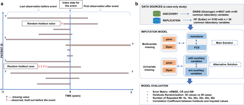
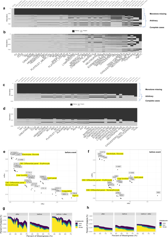
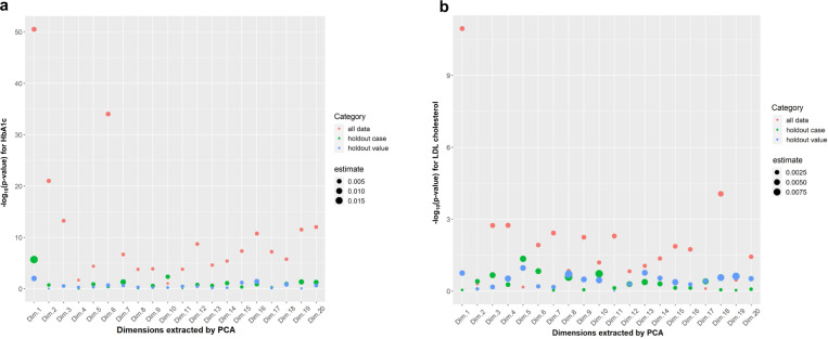
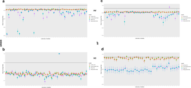
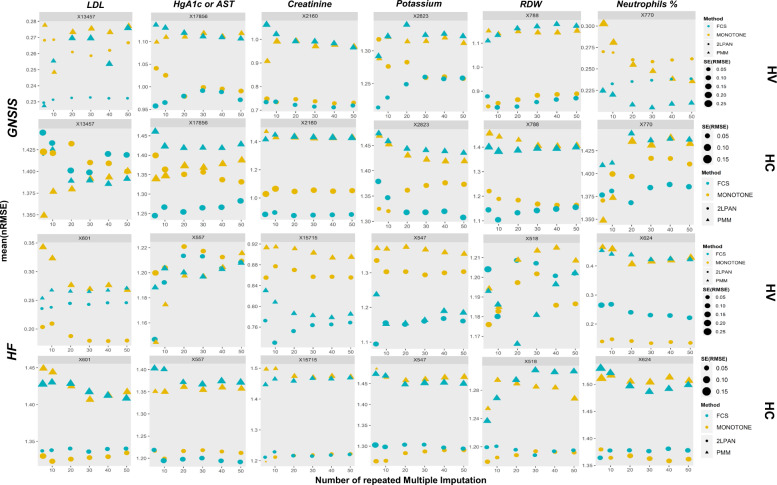
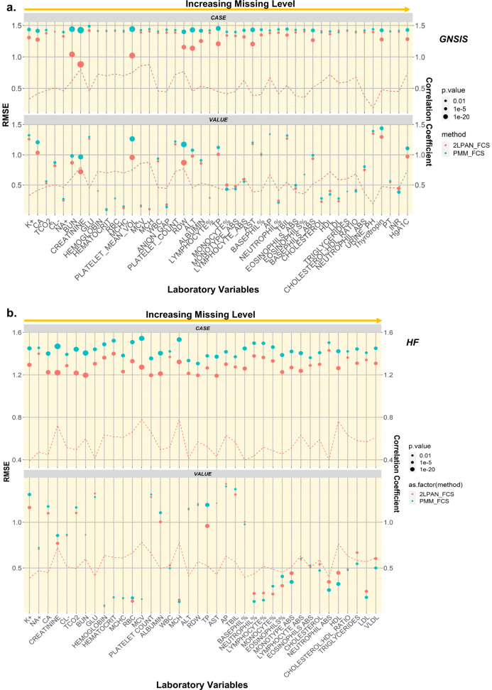
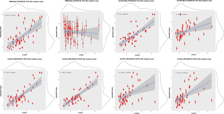
Laboratory data from Electronic Health Records (EHR) are often used in prediction models where estimation bias and model performance from missingness can be mitigated using imputation methods. We demonstrate the utility of imputation in two real-world EHR-derived cohorts of ischemic stroke from Geisinger and of heart failure from Sutter Health to: (1) characterize the patterns of missingness in laboratory variables; (2) simulate two missing mechanisms, arbitrary and monotone; (3) compare cross-sectional and multi-level multivariate missing imputation algorithms applied to laboratory data; (4) assess whether incorporation of latent information, derived from comorbidity data, can improve the performance of the algorithms. The latter was based on a case study of hemoglobin A1c under a univariate missing imputation framework. Overall, the pattern of missingness in EHR laboratory variables was not at random and was highly associated with patients’ comorbidity data; and the multi-level imputation algorithm showed smaller imputation error than the cross-sectional method.
Overview
The claims and statistics of this paper haven’t been checked yet.
Run the check — free, no account needed. It reads the open-access text and checks the sources it cites.
Integrity signals
Registry
Cites
Statistics
Figures
Verification
Claims the paper makes
The claims and statistics of this paper haven’t been checked yet.
Run the check — free, no account needed. It reads the open-access text and checks the sources it cites.
Self-check
Percentages, sums and reported differences re-computed from the paper’s own numbers.
The self-check needs the paper’s full text.
Citations
Cites
Maximum Likelihood from Incomplete Data Via the EM Algorithm
Dempster, A. P., Laird, N. M., & Rubin, D. B. (1977) · Journal of the Royal Statistical Society Series B: Statistical Methodology · doi:10.1111/j.2517-6161.1977.tb01600.x · Cited by 50,444
Multiple Imputation for Nonresponse in Surveys
Rubin, D. B. (1987) · Wiley Series in Probability and Statistics · doi:10.1002/9780470316696 · Cited by 20,701
mice: Multivariate Imputation by Chained Equations in R
Buuren, S. V., & Groothuis-Oudshoorn, K. (2011) · Journal of Statistical Software · doi:10.18637/jss.v045.i03 · Cited by 13,870
Grundy, S. M., Cleeman, J. I., Daniels, S. R., Donato, K. A., Eckel, R. H., Franklin, B. A., Gordon, D. J., Krauss, R. M., Savage, P. J., Smith, S. C., et al. (2005) · Circulation · doi:10.1161/circulationaha.105.169404 · Cited by 11,961
RUBIN, D. B. (1976) · Biometrika · doi:10.1093/biomet/63.3.581 · Cited by 9,925
Analysis of Incomplete Multivariate Data
Schafer, J. L. (1997) · doi:10.1201/9781439821862 · Cited by 6,012
Analysis of Incomplete Multivariate Data
Booth, D. E., & Schafer, J. L. (2000) · Technometrics · doi:10.2307/1271466 · Cited by 5,627
Multiple imputation of discrete and continuous data by fully conditional specification
van Buuren, S. (2007) · Statistical Methods in Medical Research · doi:10.1177/0962280206074463 · Cited by 2,827
Flexible Imputation of Missing Data, Second Edition
van Buuren, S. (2018) · doi:10.1201/9780429492259 · Cited by 2,273
A multivariate technique for multiply imputing missing values using a sequence of regression models
Raghunathan, T. E., Lepkowski, J. M., Hoewyk, J. V., & Solenberger, P. W. (2001) · Survey methodology · Cited by 1,981
Research works printed but not linked: 2
- Ford, B. in Incomplete Data in Sample Surveys, Theory and Bibliographies Vol. 2 (Part IV) (eds. W. Madow, H. Nisselson, & I. Olkin) 185–207 (Academic Press, 1983).
- Van Buuren, S. & Groothuis-Oudshoorn, K. mice: multivariate imputation by chained equations in R. J. Stat. Softw. 45, 67 (2011). · DOI · Paper page
Cited by
Sorted by citations
Acosta, J. N., Falcone, G. J., Rajpurkar, P., & Topol, E. J. (2022) · Nature Medicine · doi:10.1038/s41591-022-01981-2 · Cited by 1,365
Multimodal data fusion for cancer biomarker discovery with deep learning
Steyaert, S., Pizurica, M., Nagaraj, D., Khandelwal, P., Hernandez-Boussard, T., Gentles, A. J., & Gevaert, O. (2023) · Nature Machine Intelligence · doi:10.1038/s42256-023-00633-5 · Cited by 402
Challenges in and Opportunities for Electronic Health Record-Based Data Analysis and Interpretation
Kim, M. K., Rouphael, C., McMichael, J. P., Welch, N., & Dasarathy, S. (2023) · Gut and Liver · doi:10.5009/gnl230272 · Cited by 142
Designing a feature selection method based on explainable artificial intelligence
Zacharias, J., von Zahn, M., Chen, J., & Hinz, O. (2022) · Electronic Markets · doi:10.1007/s12525-022-00608-1 · Cited by 109
Detecting and Remediating Harmful Data Shifts for the Responsible Deployment of Clinical AI Models
Subasri, V., Krishnan, A., Kore, A., Dhalla, A., Pandya, D., Wang, B., Malkin, D., Razak, F., Verma, A. A., Goldenberg, A., et al. (2025) · JAMA Network Open · doi:10.1001/jamanetworkopen.2025.13685 · Cited by 87
Biases in Electronic Health Records Data for Generating Real-World Evidence: An Overview
Al‐Sahab, B., Leviton, A., Loddenkemper, T., Paneth, N., & Zhang, B. (2023) · Journal of Healthcare Informatics Research · doi:10.1007/s41666-023-00153-2 · Cited by 77
Ren, W., Liu, Z., Wu, Y., Zhang, Z., Hong, S., Liu, H., & on behalf of the Missing Data in Electronic health Records (MINDER) Group (2024) · Health Data Science · doi:10.34133/hds.0176 · Cited by 54
Lin, X., Liang, C., Liu, J., Lyu, T., Ghumman, N., & Campbell, B. A. (2024) · Journal of Medical Internet Research · doi:10.2196/54737 · Cited by 69
Bernardini, M., Doinychko, A., Romeo, L., Frontoni, E., & Amini, M.-R. (2023) · Computers in Biology and Medicine · doi:10.1016/j.compbiomed.2023.107188 · Cited by 42
An open-source framework for end-to-end analysis of electronic health record data
Heumos, L., Ehmele, P., Treis, T., zu Belzen, J. U., Roellin, E., May, L., Namsaraeva, A., Horlava, N., Shitov, V. A., Zhang, X., et al. (2024) · Nature Medicine · doi:10.1038/s41591-024-03214-0 · Cited by 52
Chen, R. K., Petrazzini, B. O., Malick, W. A., Rosenson, R. S., & Do, R. (2023) · Arteriosclerosis Thrombosis and Vascular Biology · doi:10.1161/atvbaha.123.320331 · Cited by 34
Minimizing bias when using artificial intelligence in critical care medicine
Ranard, B. L., Park, S., Jia, Y., Zhang, Y., Alwan, F. S., Celi, L. A., & Lusczek, E. R. (2024) · Journal of Critical Care · doi:10.1016/j.jcrc.2024.154796 · Cited by 27
Kapral, L., Dibiasi, C., Jeremic, N., Bartos, S., Behrens, S., Bilir, A., Heitzinger, C., & Kimberger, O. (2024) · EClinicalMedicine · doi:10.1016/j.eclinm.2024.102797 · Cited by 33
Wang, Z., Chen, S., Liu, T., & Yao, B. (2024) · IEEE Journal of Biomedical and Health Informatics · doi:10.1109/jbhi.2024.3351949 · Cited by 31
Digitale, J. C., Franzon, D. E., Pletcher, M. J., McCulloch, C. E., & Gennatas, E. D. (2025) · JMIR Medical Informatics · doi:10.2196/79307 · Cited by 30
Exploring Machine Learning Applications in Pediatric Asthma Management: Scoping Review
Ojha, T., Patel, A., Sivapragasam, K., Sharma, R., Vosoughi, T., Skidmore, B., Pinto, A. D., & Hosseini, B. (2024) · JMIR AI · doi:10.2196/57983 · Cited by 25
Lifting Hospital Electronic Health Record Data Treasures: Challenges and Opportunities
Maletzky, A., Böck, C., Tschoellitsch, T., Roland, T., Ludwig, H., Thumfart, S., Giretzlehner, M., Hochreiter, S., & Meier, J. M. (2022) · JMIR Medical Informatics · doi:10.2196/38557 · Cited by 23
Opportunities and challenges for biomarker discovery using electronic health record data
Singhal, P., Tan, A. L. M., Drivas, T. G., Johnson, K. B., Ritchie, M. D., & Beaulieu-Jones, B. K. (2023) · Trends in Molecular Medicine · doi:10.1016/j.molmed.2023.06.006 · Cited by 21
Wang, M., Kuo, Y., Kuo, L.-C., Liang, H.-P., Cheng, Y., Yeh, Y.-C., Tsai, M.-T., Chan, W.-S., Chiu, C., Chao, A., et al. (2023) · Journal of Clinical Anesthesia · doi:10.1016/j.jclinane.2023.111121 · Cited by 20
Tsiampalis, T., & Panagiotakos, D. B. (2023) · BMC Medical Research Methodology · doi:10.1186/s12874-023-02004-5 · Cited by 24
Artificial Intelligence and Machine Learning in Transfusion Practice: An Analytical Assessment
Li, N., Goel, R., Raza, S., Riazi, K., Pan, J., Nguyen, H. Q., Shih, A. W. Y., D’Souza, A. G., Dubey, R., Tobian, A. A. R., et al. (2025) · Transfusion Medicine Reviews · doi:10.1016/j.tmrv.2025.150926 · Cited by 17
Incompleteness of Electronic Health Records: An Impending Process Problem Within Healthcare
Gurupur, V. P., Hooshmand, S., Prabhu, D. F., Trader, E. A., & Salvi, S. (2025) · Healthcare · doi:10.3390/healthcare13222900 · Cited by 22
Zhou, S., Blaes, A. H., Shenoy, C., Sun, J., & Zhang, R. (2024) · iScience · doi:10.1016/j.isci.2024.110329 · Cited by 17
Artificial Intelligence: A Shifting Paradigm in Cardio-Cerebrovascular Medicine
Abedi, V., Razavi, S., Khan, A., Avula, V., Tompe, A. P., Poursoroush, A., Sadr, A. V., Li, J., & Zand, R. (2021) · Journal of Clinical Medicine · doi:10.3390/jcm10235710 · Cited by 17
Self-citationOpening the Precision Diabetes Care through Digital Healthcare
Lee, J., Yu, J. S., & Yoon, K. (2023) · Diabetes & Metabolism Journal · doi:10.4093/dmj.2022.0386 · Cited by 12
A comprehensive survey of imputation methods in medical missing data analysis
Benhamza, K., Benselim, R., Naidja, H., & Séridi, H. (2025) · Applied Intelligence · doi:10.1007/s10489-025-06602-2 · Cited by 14
Data Imputation in Healthcare Applications
Nayak, S., & Khilar, P. M. (2024) · Advances in healthcare information systems and administration book series · doi:10.4018/979-8-3693-7452-8.ch004 · Cited by 11
Li, N., Riazi, K., Pan, J., Thavorn, K., Ziegler, J., Rochwerg, B. N., Quan, H., Prescott, H. C., Dodek, P., Li, B., et al. (2025) · Intensive Care Medicine Experimental · doi:10.1186/s40635-025-00744-w · Cited by 11
Incorporating informatively collected laboratory data from EHR in clinical prediction models
Sun, M., Engelhard, M., Bedoya, A., & Goldstein, B. A. (2024) · BMC Medical Informatics and Decision Making · doi:10.1186/s12911-024-02612-1 · Cited by 10
Kurvits, S., Harro, A., Reigo, A., Ott, A., Laur, S., Särg, D., Tampuu, A., Alasoo, K., Vilo, J., Milani, L. A., et al. (2023) · European journal of medical research · doi:10.1186/s40001-023-01087-6 · Cited by 10
Studying missingness in spinal cord injury data: challenges and impact of data imputation
Bourguignon, L., Lukas, L. P., Guest, J. D., Geisler, F. H., Noonan, V. K., Curt, A. E. P., Brüningk, S. C., & Jutzeler, C. R. (2024) · BMC Medical Research Methodology · doi:10.1186/s12874-023-02125-x · Cited by 10
Imputation Strategies Under Clinical Presence: Impact on Algorithmic FairnessPreprint
Jeanselme, V., De‐Arteaga, M., Zhang, Z., Tom, B. D. M., & Barrett, J. (2023) · SSRN Electronic Journal · doi:10.2139/ssrn.4496874 · Cited by 10
Klann, J. G., Henderson, D. W., Morris, M. M., Estiri, H., Weber, G. M., Visweswaran, S., & Murphy, S. N. (2023) · Journal of the American Medical Informatics Association · doi:10.1093/jamia/ocad166 · Cited by 9
Jin, W., Hao, W., Shi, X., Fritsche, L. G., Salvatore, M., Admon, A. J., Friese, C. R., & Mukherjee, B. (2023) · Journal of Clinical Medicine · doi:10.3390/jcm12237313 · Cited by 8
Zhang, M., Zhang, X., Dai, M., Wu, L., Liu, K., Wang, H., Chen, W., Liu, M., & Hu, Y. (2024) · International Journal of Medical Informatics · doi:10.1016/j.ijmedinf.2024.105588 · Cited by 8
Quesada, J. A., & Orozco‐Beltrán, D. (2024) · International Journal of Medical Informatics · doi:10.1016/j.ijmedinf.2024.105722 · Cited by 8
Artificial intelligence in the clinical setting
Vistisen, S. T., Pollard, T., Harris, S. K., & Lauritsen, S. M. (2022) · European Journal of Anaesthesiology · doi:10.1097/eja.0000000000001696 · Cited by 7
Predicting mortality among ischemic stroke patients using pathways-derived polygenic risk scores
Li, J., Chaudhary, D. P., Griessenauer, C. J., Carey, D. J., Zand, R., & Abedi, V. (2022) · Scientific Reports · doi:10.1038/s41598-022-16510-x · Cited by 7
Self-citationIncreasing efficiency of SVMp+ for handling missing values in healthcare prediction
Zhang, Y., Gao, Z., Wittrup, E. M., Gryak, J., & Najarian, K. (2023) · PLOS Digital Health · doi:10.1371/journal.pdig.0000281 · Cited by 7
Machine Learning-Based Prediction of Stroke in Emergency Departments
Abedi, V., Misra, D., Chaudhary, D. P., Avula, V., Schirmer, C. M., Li, J., & Zand, R. (2024) · Therapeutic Advances in Neurological Disorders · doi:10.1177/17562864241239108 · Cited by 7
Self-citationDefining the Age of Young Ischemic Stroke Using Data-Driven Approaches
Abedi, V., Lambert, C., Chaudhary, D., Rieder, E., Avula, V., Hwang, W., Li, J., & Zand, R. (2023) · Journal of Clinical Medicine · doi:10.3390/jcm12072600 · Cited by 7
Self-citationLiao, W., Zhu, Y., Zhang, Z., Wang, Y., Wang, Z., Chu, X., Wang, Y., & Ma, L. (2025) · ACM SIGKDD Conference on Knowledge Discovery and Data Mining (KDD) · doi:10.1145/3690624.3709166 · Cited by 8
How Deep is Your Guess? A Fresh Perspective on Deep Learning for Medical Time-Series Imputation
Qian, L., Ellis, H. L., Wang, T., Wang, J., Mitra, R., Dobson, R., & Ibrahim, Z. M. (2025) · IEEE Journal of Biomedical and Health Informatics · doi:10.1109/jbhi.2025.3568778 · Cited by 11
Boie, S. D., Engelhardt, L. J., Coenen, N., Giesa, N., Rubarth, K., Menk, M., & Balzer, F. (2022) · JMIR Medical Informatics · doi:10.2196/39187 · Cited by 6
Toumi, S., Aljadani, A., Toumi, H., Ammouri, B., & Dhiabi, M. (2025) · Eurasian economic review : · doi:10.1007/s40822-024-00295-7 · Cited by 9
Flexible imputation toolkit for electronic health records
Sadr, A. V., Li, J., Hwang, W., Yeasin, M., Wang, M., Lehmann, H. P., Zand, R., & Abedi, V. (2025) · Scientific Reports · doi:10.1038/s41598-025-02276-5 · Cited by 9
Self-citationAbass, S. A. E., Altamimi, A. S. A., Aldakhil, T., & Prajapati, P. (2026) · Critical Reviews in Analytical Chemistry · doi:10.1080/10408347.2026.2694610 · Cited by 6
Hejazian, S. S., Sadr, A. V., Shahjouei, S., Vemuri, A. K., Zhou, S., Abedi, V., & Zand, R. (2024) · Journal of Stroke and Cerebrovascular Diseases · doi:10.1016/j.jstrokecerebrovasdis.2024.108007 · Cited by 6
Self-citationHe, H., Zhao, H., Li, L., Yang, H. B., Yan, J., Yuan, Y., Hu, X., & Zhang, Y. (2025) · Computer Methods and Programs in Biomedicine · doi:10.1016/j.cmpb.2025.108618 · Cited by 5
Missing Values in Longitudinal Proteome Dynamics Studies: Making a Case for Data Multiple Imputation
Yan, Y., Sankar, B. S., Mirza, B., Ng, D. C. M., Pelletier, A. R., Huang, S. D., Wang, W. W., Watson, K. E., Wang, D., & Ping, P. (2024) · Journal of Proteome Research · doi:10.1021/acs.jproteome.4c00263 · Cited by 5
Salvatore, M., Kundu, R., Du, J., Friese, C. R., Mondul, A. M., Hanauer, D. A., Lu, H., Pearce, C. L., & Mukherjee, B. (2024) · medRxiv · doi:10.1101/2024.10.28.24316286 · Cited by 8
Ma, L., Yang, L., Wang, Y., Hao, J., Li, Y., Ma, L., Wang, Z., Li, Y., Zhang, S., Hu, M., et al. (2025) · Digital Health · doi:10.1177/20552076251352436 · Cited by 4
Self-citationOh, M., Kim, H.-S., Jung, Y. M., Lee, H.-C., Lee, S.-B., & Lee, S. M. (2025) · Scientific Reports · doi:10.1038/s41598-025-24826-7 · Cited by 4
Orozco‐Beltrán, D., Seidu, S., & Quesada, J. A. (2025) · Primary care diabetes · doi:10.1016/j.pcd.2025.11.012 · Cited by 4
Children’s Physical Activity during COVID-19 in Ontario, Canada: Parents’ Perspectives
Szpunar, M., Saravanamuttoo, K., Vanderloo, L. M., Bruijns, B. A., Truelove, S., Burke, S. M., Gilliland, J., Irwin, J. D., & Tucker, P. (2022) · International Journal of Environmental Research and Public Health · doi:10.3390/ijerph192215061 · Cited by 4
Patient Event Sequences for Predicting Hospitalization Length of Stay
Hansen, E. R., Nielsen, T. D., Mulvad, T., Stausholm, M. N., Sagi, T., & Hose, K. (2023) · Lecture notes in computer science · doi:10.1007/978-3-031-34344-5_7 · Cited by 5
Prediction of postoperative infections by strategic data imputation and explainable machine learning
Guillen-Ramirez, H., Sánchez‐Taltavull, D., Perrodin, S. F., Peisl, S., Triep, K., Gaudet-Blavignac, C., Endrich, O., & Beldi, G. (2025) · Journal of the American Medical Informatics Association · doi:10.1093/jamia/ocaf145 · Cited by 3
Wearable device-measured circadian rest–activity rhythm with mortality risk in patients with cancer
Mei, X., Zheng, N., Li, B., Liu, Y., Yang, L., Luo, T., Chan, N. Y., Chan, J. W. Y., Liu, Y., Tan, X. W., et al. (2025) · BMJ Health & Care Informatics · doi:10.1136/bmjhci-2025-101553 · Cited by 5
Laeeq, A., Li, J., & Adeel, U. (2026) · Machine Learning and Knowledge Extraction · doi:10.3390/make8010018 · Cited by 6
Self-citationThangaraj, P., Oikonomou, E. K., Dhingra, L. S., Aminorroaya, A., Jayaram, R. H., Suchard, M. A., & Khera, R. (2025) · Circulation Cardiovascular Quality and Outcomes · doi:10.1161/circoutcomes.124.011306 · Cited by 3
The health-related quality of life among survivors with post-COVID conditions in the United States
Hejazian, S. S., Vemuri, A. K., Sadr, A. V., Shahjouei, S., Bahrami, S., Zhou, S., Abedi, V., & Zand, R. (2025) · PLoS ONE · doi:10.1371/journal.pone.0320721 · Cited by 3
Self-citationLiang, C., Weissman, S., Olatosi, B., Poon, E. G., Yarrington, M. E., & Li, X. (2022) · BMJ Open · doi:10.1136/bmjopen-2022-067204 · Cited by 3
Shehhi, A. A., Almansoori, T. M., Alsuwaidi, A. R., & Alblooshi, H. (2024) · PLoS ONE · doi:10.1371/journal.pone.0291373 · Cited by 3
Enhanced Optimized Classification Model of Chronic Kidney Disease
Elkholy, S., Rezk, A., & Saleh, A. A. E. F. (2023) · International Journal of Advanced Computer Science and Applications · doi:10.14569/ijacsa.2023.0140239 · Cited by 3
Focal Loss Improves Performance of High-Sensitivity C-Reactive Protein Imbalanced Classification
Sledzik, R., & Zabihimayvan, M. (2022) · Proceedings - IEEE Symposium on Computer-Based Medical Systems · doi:10.1109/cbms55023.2022.00027 · Cited by 4
Chavoshian, S., Fossat, Y., Cao, X., Kaufman, J. M., Stanbrook, M. B., Tarlo, S. M., & Yadollahi, A. (2025) · IEEE Journal of Biomedical and Health Informatics · doi:10.1109/jbhi.2025.3582739 · Cited by 2
A Hybrid LSTM-Attention Approach for Missing Data Imputation in IoT Time Series
Laeeq, A., Adeel, U., Li, J., & Starkey, E. (2025) · Lecture notes in computer science · doi:10.1007/978-3-032-10486-1_28 · Cited by 2
Self-citationMissing Value Imputation in Tabular Data Lakes Unleashed: A Hybrid Approach
Luo, F., Lan, H., Luo, H., Bao, Z., Culpepper, J. S., Sadiq, S. W., & Wang, X. (2026) · The VLDB Journal · doi:10.1007/s00778-025-00957-1 · Cited by 2
Hejazian, S. S., Vemuri, A. K., Sadr, A. V., Shahjouei, S., Bahrami, S., Abedi, V., & Zand, R. (2025) · Journal of Stroke and Cerebrovascular Diseases · doi:10.1016/j.jstrokecerebrovasdis.2025.108246 · Cited by 2
Self-citationGupta, S., Sharma, S., Sharma, R. K., & Chandra, J. (2025) · Artificial Intelligence in Medicine · doi:10.1016/j.artmed.2025.103134 · Cited by 3
A Self-Supervised Framework for Laboratory Data Imputation in Electronic Health Records
Heilbroner, S. P., Carter, C., Vidmar, D. M., Mueller, E. T., Stumpe, M. C., & Miotto, R. (2025) · Communications Medicine · doi:10.1038/s43856-025-00973-w · Cited by 1
Faes, L., Mishra, A. V., Lipkova, V., Balaskas, K., Quek, C. W. N., HAMILTON, R. D., Held, U., Sim, D. A., Sivaprasad, S., & Fu, D. J. (2023) · Journal of Clinical Medicine · doi:10.3390/jcm12123878 · Cited by 1
lab: an R package for generating analysis-ready data from laboratory records
Tseng, Y., Chen, C. J., & Chang, C. W. (2023) · PeerJ Computer Science · doi:10.7717/peerj-cs.1528 · Cited by 1
Disparities in perceived general health of stroke survivors in the United States
Hejazian, S. S., Sadr, A. V., Vemuri, A. K., Abedi, V., & Zand, R. (2025) · Journal of the Neurological Sciences · doi:10.1016/j.jns.2025.123556 · Cited by 1
Self-citationHou, Z., Zhao, Z., Zhu, D., Pan, M., Zhou, Y., & Ge, Q. (2025) · International Symposium on Intelligent Robotics and Systems (ISoIRS) · doi:10.1109/isoirs65690.2025.11167916 · Cited by 1
Five-year dementia prediction and decision support system based on real-world data
Exarchos, T. P., Dimakopoulos, G. A., Lazaros, K., Krokidis, M. G., Vrahatis, A. G., Grammenos, G., Avramouli, A., Skolariki, K., Adams, R., Mahairaki, V., et al. (2025) · Frontiers in Aging Neuroscience · doi:10.3389/fnagi.2025.1670609 · Cited by 1
Integrated analysis for electronic health records with structured and sporadic missingness
Tan, J., Zhang, Y., Hong, C., Cai, T. T., Cai, T., & Zhang, A. R. (2025) · Journal of Biomedical Informatics · doi:10.1016/j.jbi.2025.104933 · Cited by 2
Garssen, S. H., Wesselink, S. F. O., Doggen, C. J. M., Koning, M. V., Veldkamp, B. P., & Haeri, M. A. (2025) · Intelligent Medicine · doi:10.1016/j.imed.2025.12.010 · Cited by 1
Cerimagic, T., Sosnin, S. D., & Ecker, G. F. (2026) · Digital Discovery · doi:10.1039/d5dd00536a · Cited by 2
Sreenivasan, M., Madhavendranath, S., & Chacko, A. M. (2026) · Biomedical Physics & Engineering Express · doi:10.1088/2057-1976/ae38de · Cited by 1
Knowledge-enhanced AI models for domain-specific application: a survey
Li, X.-Y., Wang, Y., Liang, J., Wang, X., Zhou, P., Zhao, Q., Zhang, Y., & Song, Q. (2026) · Science China Information Sciences · doi:10.1007/s11432-025-4635-0 · Cited by 1
Multiple Imputation of a Continuous Outcome with Fully Observed Predictors Using TabPFN
Sepin, J. (2026) · Stats · doi:10.3390/stats9020038 · Cited by 1
Towards Explainable Hospital Mortality Prediction Using Critical Care Data
Ali, M. S., & Mahmud, M. (2026) · Lecture notes in computer science · doi:10.1007/978-3-032-29842-3_29 · Cited by 1
Giesa, N., Zhumagambetov, R., Sekutowitcz, M., Piper, S. K., Sikora, V., Balzer, F., Haufe, S., & Boie, S. D. (2026) · Nature Communications · doi:10.1038/s41467-026-77303-8 · Cited by 2
Garssen, S. H., Vernooij, C. A., Kant, N., Koning, M. V., Bosch, F. H., Doggen, C. J. M., Veldkamp, B. P., Verhaegh, W., & Wesselink, S. F. O. (2024) · International Journal of Medical Informatics · doi:10.1016/j.ijmedinf.2024.105586 · Cited by 1
Similarity-Based Prediction of Ejection Fraction in Heart Failure Patients
Wallis, J., Azqueta-Gavaldón, A., Ananthakumar, T., Dürichen, R., & Albergante, L. (2022) · Informatics in Medicine Unlocked · doi:10.1016/j.imu.2022.101035
Boie, S. D., Engelhardt, L. J., Coenen, N., Giesa, N., Rubarth, K., Menk, M., & Balzer, F. (2022) · doi:10.2196/preprints.39187
Curier, L., Brouwer, C. G., wardak, H., van Twist, D. J. L., Bromuri, S., Martens, R. J. H., & Leers, M. P. G. (2023) · Research Square · doi:10.21203/rs.3.rs-3181908/v1
Li, J., Abedi, V., & Zand, R. (2023) · Mayo Clinic Proceedings Digital Health · doi:10.1016/j.mcpdig.2023.06.009
Self-citationRepresenting Health Data and Medical Knowledge for Deep Learning
Hansen, E. R. (2023) · VBN Forskningsportal (Aalborg Universitet) · doi:10.54337/aau621651364
Data analytics framework for sparse longitudinal structured biomedical data
Sixtová, I., Skopal, T., & Uher, T. (2023) · IEEE International Conference on Bioinformatics and Biomedicine (BIBM) · doi:10.1109/bibm58861.2023.10385940
Çabuk, U. C., & Öztürk, Y. (2024) · ASEE Pacific Southwest Section Conference (PSW) · doi:10.18260/1-2--46017
Prediction of postoperative infections by strategic data imputation and explainable machine learningPreprint
Beldi, G., Guillen-Ramirez, H., Sánchez‐Taltavull, D., Perrodin, S. F., Triep, K., & Endrich, O. (2024) · Research Square · doi:10.21203/rs.3.rs-4594014/v1
Theocharopoulos, P. C., Bersimis, S., Georgakopoulos, S. V., Plagianakos, V. P., & Tasoulis, S. K. (2025) · doi:10.1109/cihm64979.2025.10969489
A probabilistic approach for building disease phenotypes across electronic health records
Vidmar, D., Freitas, J. D., Thompson, W., Pfeifer, J. M., Fornwalt, B. K., Zimmerman, N., Miotto, R., & Chen, R. (2025) · BioData Mining · doi:10.1186/s13040-025-00454-9
Comparison of Imputation Strategies for Incomplete Electronic Health Data
Zhang, S., Zhang, Z., Zhou, Y., Hong, S., & Liu, H. (2026) · Health Data Science · doi:10.34133/hds.0493
Enhanced multi-task learning of imputation and prediction via feature relationship graph learningPreprint
Hur, S.-W., Lee, T.-H., & Jun, C. (2025) · SSRN Electronic Journal · doi:10.2139/ssrn.5473084
Charvadeh, Y. K., Seier, K. P., Panageas, K. S., Vaithilingam, D., Gönen, M., & Chen, Y. (2025) · Statistics in Medicine · doi:10.1002/sim.70335
A New Robust Imputation Method for Longitudinal Data with Non-Normal Continuous Outcomes
Darwish, N. M., Mohamed, Y. A., Gad, A. M., Abd-Rabou, A.-E. S., & Ibrahim, W. M. (2025) · International Journal of Statistics in Medical Research · doi:10.6000/1929-6029.2025.14.70
Multimorbidity measurement strategies for predicting hospital visits
Neves, B. D., Moreira, J. M., Gonçalves, S., Cerejo, J., Mota, I., Silva, N. A., Leite, F., & Silva, M. J. (2025) · BMC Health Services Research · doi:10.1186/s12913-025-13817-z
Metadata
- Authors
- Li, J., Yan, X. S., Chaudhary, D., Avula, V., Mudiganti, S., Husby, H., Shahjouei, S., Afshar, A., Stewart, W. F., Yeasin, M., Zand, R., & Abedi, V.
- Affiliations
- Geisinger Health System (US)
- Sutter Health (US)
- Georgia Institute of Technology (US)
- University of Memphis (US)
- Pennsylvania State University (US)
- Corresponding author
- Abedi, Vida
- ORCID
- Venue
- npj Digital Medicine
- Published
- 2021-10-11
- Volume
- 4
- Issue
- 1
- Pages
- 147-147
- ISSN
- 2398-6352 (ISSN-L)
- PMC
- PMC8505441
- OpenAlex
- W3205484571
- Cited by
- 133
- References
- 47
- Citations by year
- 2026: 30 · 2025: 35 · 2024: 33 · 2023: 23 · 2022: 11 · 2021: 1
- FWCI
- 12.68
- Type
- journal article
- Language
- en
- Open access
- gold
- doi.org
- Locations
- npj Digital Medicine (publishedVersion, cc-by)
- Europe PMC (PubMed Central) (publishedVersion, other-oa)
- PubMed Central (publishedVersion, cc-by)
- PubMed (publishedVersion)
- DOAJ (DOAJ: Directory of Open Access Journals) (submittedVersion, cc-by-sa)
- Funders
- U.S. Department of Health & Human Services | NIH | Center for Information Technology (R56HL116832)
- Topics
- Physical Sciences › Mathematics › Statistics and Probability › Statistical Methods and Bayesian Inference
- Physical Sciences › Computer Science › Artificial Intelligence › Machine Learning in Healthcare
- Health Sciences › Health Professions › Health Information Management › Artificial Intelligence in Healthcare
- Keywords
- missing data imputation, electronic health records, laboratory findings, ischemic stroke, heart failure, missingness patterns, comorbidities, HbA1c, imputation error
About these checks
Registry, retraction, Cites and statistics results are computed, not judged, with one exception: a printed reference that no index lists is read once by a model before it counts as a citation error. Claims are extracted by a model and kept only when their quote appears verbatim in the text; each cited source is then checked, with a model’s help, for whether it says what the claim relies on. Those verdicts can be wrong — read the claim’s quote and the cited source before relying on one.
Statistics and arithmetic are recomputed, not judged.
Confidence bands are shown only for fields calibrated on our annotated test set. None is calibrated yet, so no band is shown.
What counts as a claim ›How we measure confidence ›How we check this ›
Are you an author, or do you see a problem with this page? Request a review
