

The DOI matches its Crossref record; 72 of the 73 references it cites were found in a registry or an index.
Chimera: enabling hierarchy based multi-objective optimization for self-driving laboratories
Open accessPublished version of a preprint
Abstract
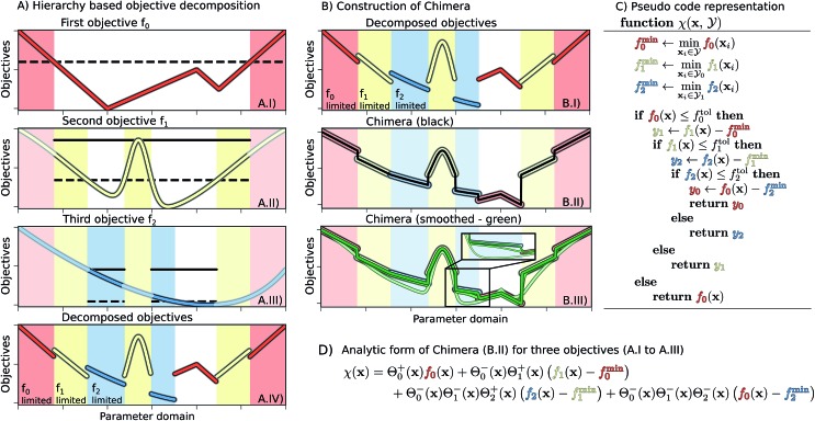
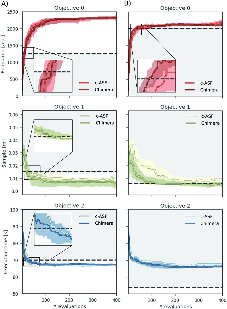
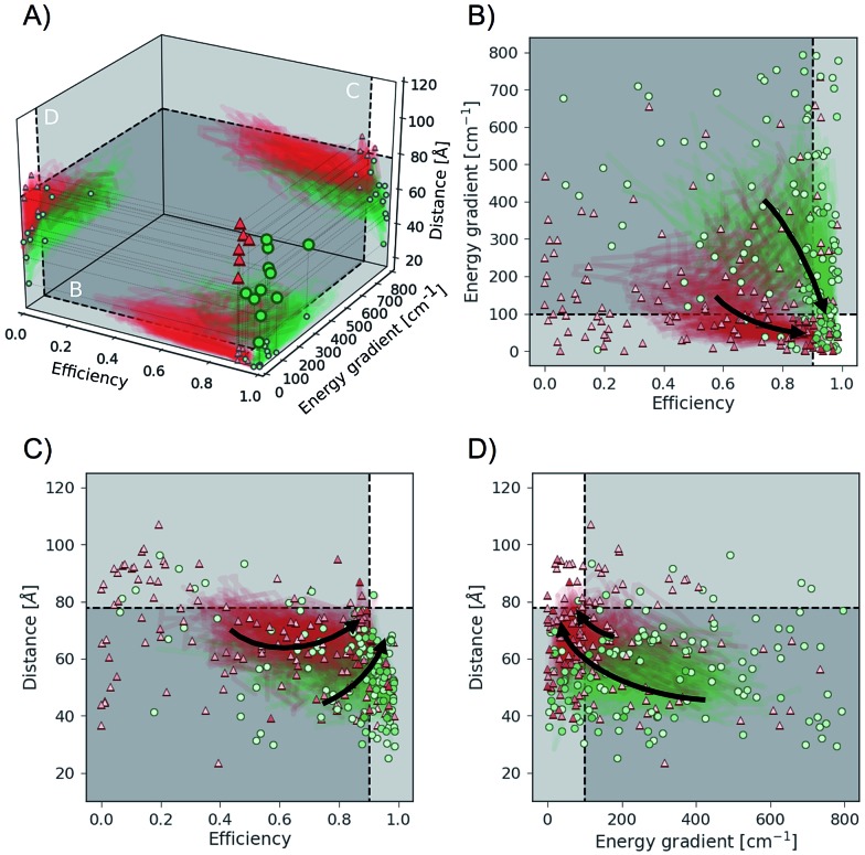
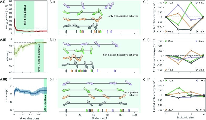
Chimera enables multi-target optimization for experimentation or expensive computations, where evaluations are the limiting factor.
Overview
The claims and statistics of this paper haven’t been checked yet.
Run the check — free, no account needed. It reads the open-access text and checks the sources it cites.
Integrity signals
Registry
Cites
Statistics
Figures
Verification
Claims the paper makes
The claims and statistics of this paper haven’t been checked yet.
Run the check — free, no account needed. It reads the open-access text and checks the sources it cites.
Claims other papers make about this one
Each is checked against this paper’s own text: does it say what the citing paper says it does?
In the citing paper
“A mathematical function called CHIMERA was recently introduced to address these problems;169 it can be used with any optimizer, such as PHOENICS.”
From QSAR without borders (2020) · cites this paper as [169]
Self-check
Percentages, sums and reported differences re-computed from the paper’s own numbers.
The self-check needs the paper’s full text.
Citations
Cites
A fast and elitist multiobjective genetic algorithm: NSGA-II
Deb, K., Pratap, A., Agarwal, S., & Meyarivan, T. (2002) · IEEE Transactions on Evolutionary Computation · doi:10.1109/4235.996017 · Cited by 50,053
A Simplex Method for Function Minimization
Nelder, J. A., & Mead, R. (1965) · The Computer Journal · doi:10.1093/comjnl/7.4.308 · Cited by 28,905
Multiple Attribute Decision Making: Methods and Applications
Chen, S.-J. J., Hwang, C. L., Beckmann, M. J., & Krelle, W. E. (1981) · Medical Entomology and Zoology · Cited by 8,207
Nonlinear Multiobjective Optimization
Miettinen, K. (1998) · International series in management science/operations research/International series in operations research & management science · doi:10.1007/978-1-4615-5563-6 · Cited by 4,994
Survey of multi-objective optimization methods for engineering
Marler, R. T., & Arora, J. S. (2004) · Structural and Multidisciplinary Optimization · doi:10.1007/s00158-003-0368-6 · Cited by 4,760
Completely Derandomized Self-Adaptation in Evolution Strategies
Hansen, N., & Ostermeier, A. (2001) · Evolutionary Computation · doi:10.1162/106365601750190398 · Cited by 4,397
Das, I., & Dennis, J. E. (1998) · SIAM Journal on Optimization · doi:10.1137/s1052623496307510 · Cited by 2,677
Hansen, N., Müller, S. D., & Koumoutsakos, P. (2003) · Evolutionary Computation · doi:10.1162/106365603321828970 · Cited by 2,601
An Overview of Evolutionary Algorithms in Multiobjective Optimization
Fonseca, C. M., & Fleming, P. J. (1995) · Evolutionary Computation · doi:10.1162/evco.1995.3.1.1 · Cited by 2,258
Multiobjective Programming and Planning
(1978) · Mathematics in Science and Engineering/Mathematics in science and engineering · doi:10.1016/s0076-5392(08)x6053-9 · Cited by 2,035
Research works printed but not linked: 14
- M. Awad and R.Khanna , in Multiobjective Optimization , Apress , Berkeley, CA , 2015 , pp. 185–208
- L. M. Roch , F.Häse , C.Kreisbeck , T.Tamayo-Mendoza , L. P. E.Yunker , J. E.Hein and A.Aspuru-Guzik , chemRxiv preprint chemRxiv:5953606 , 2018
- D. Hernández-Lobato , J.Hernandez-Lobato , A.Shah and R. P.Adams , International Conference on Machine Learning , 2016 , pp. 1492–1501
- M. Emmerich and J. W.Klinkenberg , Rapport technique , Leiden University , 2008 , vol. 34
- W. Ponweiser , T.Wagner , D.Biermann and M.Vincze , International Conference on Parallel Problem Solving from Nature , 2008 , pp. 784–794
- M. Pescador-Rojas , R. H.Gómez , E.Montero , N.Rojas-Morales , M. C.Riff and C. A.Coello , International Conference on Evolutionary Multi-Criterion Optimization , 2017 , pp. 499–513
- V. Changkong and Y. Y.Haimes , North-Holland Series in System Science and Engineering , Elsevier Science Publishing Co , New York NY , 1983 , vol. 8
- O. Grodzevich and O.Romanko , Proceedings of the Fields-MITACS Industrial Problems Workshop , 2006
- M. J. Rentmeesters , W. K.Tsai and K. J.Lin , Second IEEE International Conference on Engineering of Complex Computer Systems, 1996. Proceedings. , 1996 , pp. 76–79
- Broyden, 1970, J. Applied Math., 6, 76
- R. A. Fisher , The design of experiments , Oliver and Boyd ; Edinburgh; London , 1937
- J. Snoek , H.Larochellrobotie and R. P.Adams , Advances in Neural Information Processing Systems (NIPS) , 2012 , vol. 25 , pp. 2951–2959
- J. Snoek , K.Swersky , R.Zemel and R. P.Adams , International Conference on Machine Learning , 2014 , pp. 1674–1682
- Y. Tanimura and R.Kubo ,J. Phys. Soc. Jpn., 1989 , 58 , 101114
Cited by
Sorted by citations
Muratov, E. N., Bajorath, J., Sheridan, R. P., Tetko, I. V., Filimonov, D., Poroikov, V., Oprea, T. I., Baskin, I. I., Varnek, A., Roitberg, A., et al. (2020) · Chemical Society Reviews · doi:10.1039/d0cs00098a · Cited by 913
Self-citationSelf-driving laboratory for accelerated discovery of thin-film materials
MacLeod, B. P., Parlane, F. G. L., Morrissey, T. D., Häse, F., Roch, L. M., Dettelbach, K. E., Moreira, R., Yunker, L. P. E., Rooney, M. B., Deeth, J. R., et al. (2020) · Science Advances · doi:10.1126/sciadv.aaz8867 · Cited by 905
Self-citationSelf-Driving Laboratories for Chemistry and Materials Science
Tom, G., Schmid, S. P., Baird, S. G., Cao, Y., Darvish, K., Hao, H., Lo, S., Pablo-García, S., Rajaonson, E. M., Skreta, M., et al. (2024) · Chemical Reviews · doi:10.1021/acs.chemrev.4c00055 · Cited by 707
Self-citationBig-Data Science in Porous Materials: Materials Genomics and Machine Learning
Jablonka, K. M., Ongari, D., Moosavi, S. M., & Smit, B. (2020) · Chemical Reviews · doi:10.1021/acs.chemrev.0c00004 · Cited by 656
Self-referencing embedded strings (SELFIES): A 100% robust molecular string representation
Krenn, M., Häse, F., Nigam, A., Friederich, P., & Aspuru‐Guzik, A. (2020) · Repository KITopen (Karlsruhe Institute of Technology) · doi:10.5445/ir/1000128111 · Cited by 616
Self-citationMachine-learned potentials for next-generation matter simulations
Friederich, P., Häse, F., Proppe, J., & Aspuru‐Guzik, A. (2021) · Nature Materials · doi:10.1038/s41563-020-0777-6 · Cited by 595
Self-citationNanoparticle synthesis assisted by machine learning
Tao, H., Wu, T., Aldeghi, M., Wu, T., Aspuru‐Guzik, A., & Kumacheva, E. (2021) · Nature Reviews Materials · doi:10.1038/s41578-021-00337-5 · Cited by 583
Self-citationData-Driven Strategies for Accelerated Materials Design
Pollice, R., Gomes, G., Aldeghi, M., Hickman, R. J., Krenn, M., Lavigne, C., Lindner-D’Addario, M., Nigam, A., Ser, C. T., Yao, Z., et al. (2021) · Accounts of Chemical Research · doi:10.1021/acs.accounts.0c00785 · Cited by 490
Self-citationA Brief Introduction to Chemical Reaction Optimization
Taylor, C. J., Pomberger, A., Felton, K., Grainger, R., Barecka, M. H., Chamberlain, T. W., Bourne, R. A., Johnson, C. N., & Lapkin, A. A. (2023) · Chemical Reviews · doi:10.1021/acs.chemrev.2c00798 · Cited by 483
Next-Generation Experimentation with Self-Driving Laboratories
Häse, F., Roch, L. M., & Aspuru-Guzik, A. (2019) · Trends in Chemistry · doi:10.1016/j.trechm.2019.02.007 · Cited by 426
Self-citationNandy, A., Duan, C., Taylor, M. G., Liu, F., Steeves, A. H., & Kulik, H. J. (2021) · Chemical Reviews · doi:10.1021/acs.chemrev.1c00347 · Cited by 358
Machine learning for metabolic engineering: A review
Lawson, C. E., Martí, J. M., Radivojević, T., Jonnalagadda, S. V. R., Gentz, R., Hillson, N. J., Peisert, S., Kim, J., Simmons, B. A., Petzold, C. J., et al. (2020) · Metabolic Engineering · doi:10.1016/j.ymben.2020.10.005 · Cited by 335
Automated self-optimization, intensification, and scale-up of photocatalysis in flow
Slattery, A., Wen, Z., Tenblad, P., Sanjosé‐Orduna, J., Pintossi, D., den Hartog, T., & Noël, T. (2024) · Science · doi:10.1126/science.adj1817 · Cited by 345
Autonomous Chemical Experiments: Challenges and Perspectives on Establishing a Self-Driving Lab
Seifrid, M. T., Pollice, R., Aguilar‐Granda, A., Chan, Z. M., Hotta, K., Ser, C. T., Vestfrid, J., Wu, T., & Aspuru‐Guzik, A. (2022) · Accounts of Chemical Research · doi:10.1021/acs.accounts.2c00220 · Cited by 327
Self-citationLangner, S., Häse, F., Perea, J. D., Stubhan, T., Hauch, J., Roch, L. M., Heumueller, T., Aspuru‐Guzik, A., & Brabec, C. J. (2020) · Advanced Materials · doi:10.1002/adma.201907801 · Cited by 270
Self-citationData-science driven autonomous process optimization
Christensen, M. M., Yunker, L. P. E., Adedeji, F., Häse, F., Roch, L. M., Gensch, T., Gomes, G., Zepel, T., Sigman, M. S., Aspuru‐Guzik, A., et al. (2021) · Communications Chemistry · doi:10.1038/s42004-021-00550-x · Cited by 243
Self-citationA Multi-Objective Active Learning Platform and Web App for Reaction Optimization
Torres, J. A. G., Lau, S. H., Anchuri, P., Stevens, J. M., Tábora, J. E., Li, J., Borovika, A., Adams, R. P., & Doyle, A. G. (2022) · Journal of the American Chemical Society · doi:10.1021/jacs.2c08592 · Cited by 215
Janet, J. P., Ramesh, S., Duan, C., & Kulik, H. J. (2020) · ACS Central Science · doi:10.1021/acscentsci.0c00026 · Cited by 200
Benavides-Hernández, J., & Dumeignil, F. (2024) · ACS Catalysis · doi:10.1021/acscatal.3c06293 · Cited by 217
Deep Learning for Deep Chemistry: Optimizing the Prediction of Chemical Patterns
Cova, T. F. G. G., & Pais, A. A. C. C. (2019) · Frontiers in Chemistry · doi:10.3389/fchem.2019.00809 · Cited by 193
Häse, F., Aldeghi, M., Hickman, R. J., Roch, L. M., & Aspuru‐Guzik, A. (2021) · Applied Physics Reviews · doi:10.1063/5.0048164 · Cited by 212
Self-citationA robotic platform for the synthesis of colloidal nanocrystals
Zhao, H., Chen, W., Huang, H., Sun, Z., Chen, Z., Wu, L., Zhang, B., Lai, F., Wang, Z., Adam, M. L., et al. (2023) · Nature Synthesis · doi:10.1038/s44160-023-00250-5 · Cited by 177
Machine-learning and high-throughput studies for high-entropy materials
Huang, E., Lee, W., Singh, S. S., Kumar, P., Lee, C., Lam, T., Chin, H.-H., Lin, B., & Liaw, P. K. (2022) · Materials Science and Engineering R Reports · doi:10.1016/j.mser.2021.100645 · Cited by 171
Machine Learning in Materials Discovery: Confirmed Predictions and Their Underlying Approaches
Saal, J. E., Oliynyk, A. O., & Meredig, B. (2020) · Annual Review of Materials Research · doi:10.1146/annurev-matsci-090319-010954 · Cited by 165
ChemOS: An orchestration software to democratize autonomous discovery
Roch, L. M., Häse, F., Kreisbeck, C., Tamayo-Mendoza, T., Yunker, L. P. E., Hein, J. E., & Aspuru‐Guzik, A. (2020) · PLoS ONE · doi:10.1371/journal.pone.0229862 · Cited by 175
Self-citationMaterials Acceleration Platforms: On the way to autonomous experimentation
Flores‐Leonar, M. M., Mejía-Mendoza, L. M., Aguilar‐Granda, A., Sánchez-Lengeling, B., Tribukait, H., Amador‐Bedolla, C., & Aspuru‐Guzik, A. (2020) · Current Opinion in Green and Sustainable Chemistry · doi:10.1016/j.cogsc.2020.100370 · Cited by 155
Self-citationSelf‐Driving Platform for Metal Nanoparticle Synthesis: Combining Microfluidics and Machine Learning
Tao, H., Wu, T., Kheiri, S., Aldeghi, M., Aspuru‐Guzik, A., & Kumacheva, E. (2021) · Advanced Functional Materials · doi:10.1002/adfm.202106725 · Cited by 141
Self-citationComputer-aided multi-objective optimization in small molecule discovery
Fromer, J. C., & Coley, C. W. (2023) · Patterns · doi:10.1016/j.patter.2023.100678 · Cited by 140
Application of machine learning for advanced material prediction and design
Chan, C. H., Sun, M., & Huang, B. (2022) · EcoMat · doi:10.1002/eom2.12194 · Cited by 123
Toward autonomous laboratories: Convergence of artificial intelligence and experimental automation
Xie, Y., Sattari, K., Zhang, C., & Lin, J. (2022) · Progress in Materials Science · doi:10.1016/j.pmatsci.2022.101043 · Cited by 129
Bayesian optimization of nanoporous materials
Deshwal, A., Simon, C. M., & Doppa, J. R. (2021) · Molecular Systems Design & Engineering · doi:10.1039/d1me00093d · Cited by 122
Dotson, J. J., van Dijk, L., Timmerman, J. C., Grosslight, S., Walroth, R. C., Gosselin, F., Püntener, K., Mack, K. A., & Sigman, M. S. (2022) · Journal of the American Chemical Society · doi:10.1021/jacs.2c08513 · Cited by 119
Schrier, J., Norquist, A. J., Buonassisi, T., & Brgoch, J. (2023) · Journal of the American Chemical Society · doi:10.1021/jacs.3c04783 · Cited by 104
Bayesian optimization with known experimental and design constraints for chemistry applications
Hickman, R. J., Aldeghi, M., Häse, F., & Aspuru-Guzik, A. (2022) · Digital Discovery · doi:10.1039/d2dd00028h · Cited by 98
Self-citationBorn, J., Manica, M., Oskooei, A., Cadow, J., Markert, G., & Martínez, M. R. (2021) · iScience · doi:10.1016/j.isci.2021.102269 · Cited by 102
Autonomous intelligent agents for accelerated materials discovery
Montoya, J. H., Winther, K. T., Flores, R. A., Bligaard, T., Hummelshøj, J. S., & Aykol, M. (2020) · Chemical Science · doi:10.1039/d0sc01101k · Cited by 100
Summit: Benchmarking Machine Learning Methods for Reaction Optimisation
Felton, K., Rittig, J. G., & Lapkin, A. A. (2021) · Chemistry - Methods · doi:10.1002/cmtd.202000051 · Cited by 108
Navigating through the Maze of Homogeneous Catalyst Design with Machine Learning
Gomes, G., Pollice, R., & Aspuru‐Guzik, A. (2021) · Trends in Chemistry · doi:10.1016/j.trechm.2020.12.006 · Cited by 87
Self-citationArtificial intelligence and automation in computer aided synthesis planning
Thakkar, A., Johansson, S., Jorner, K., Buttar, D., Reymond, J., & Engkvist, O. (2020) · Reaction Chemistry & Engineering · doi:10.1039/d0re00340a · Cited by 93
Accelerated chemical science with AI
Back, S., Aspuru‐Guzik, A., Ceriotti, M., Gryn’ova, G., Grzybowski, B. A., Gu, G. H., Hein, J. E., Hippalgaonkar, K., Hormázabal, R., Jung, Y., et al. (2023) · Digital Discovery · doi:10.1039/d3dd00213f · Cited by 91
Self-citationArtificial Intelligence (AI) Workflow for Catalyst Design and Optimization
Lai, N. S., Tew, Y. S., Zhong, X., Yin, J., Li, J., Yan, B., & Wang, X. (2023) · Industrial & Engineering Chemistry Research · doi:10.1021/acs.iecr.3c02520 · Cited by 85
Olympus: a benchmarking framework for noisy optimization and experiment planning
Häse, F., Aldeghi, M., Hickman, R. J., Roch, L. M., Christensen, M., Liles, E., Hein, J. E., & Aspuru‐Guzik, A. (2021) · Machine Learning Science and Technology · doi:10.1088/2632-2153/abedc8 · Cited by 101
Self-citationAdaptive Optimization of Chemical Reactions with Minimal Experimental Information
Reker, D., Hoyt, E. A., Bernardes, G. J. L., & Rodrigues, T. (2020) · Cell Reports Physical Science · doi:10.1016/j.xcrp.2020.100247 · Cited by 89
Parallel tempered genetic algorithm guided by deep neural networks for inverse molecular design
Nigam, A., Pollice, R., & Aspuru‐Guzik, A. (2022) · Digital Discovery · doi:10.1039/d2dd00003b · Cited by 117
Self-citationWhere Nanosensors Meet Machine Learning: Prospects and Challenges in Detecting Disease X
Leong, Y. X., Tan, E. X., Leong, S. X., Koh, C. S. L., Nguyen, L. B. T., Chen, J. R. T., Xia, K., & Ling, X. Y. (2022) · ACS Nano · doi:10.1021/acsnano.2c05731 · Cited by 81
He, C., Zhang, C., Bian, T., Jiao, K., Su, W., Wu, K., & Su, A. (2023) · Processes · doi:10.3390/pr11020330 · Cited by 88
Self-Driving Laboratories for Development of New Functional Materials and Optimizing Known Reactions
Soldatov, M. A., Butova, V. V., Pashkov, D. M., Butakova, M. A., Medvedev, P. V., Chernov, A. V., & Soldatov, A. V. (2021) · Nanomaterials · doi:10.3390/nano11030619 · Cited by 75
Five High-Impact Research Areas in Machine Learning for Materials Science
Meredig, B. (2019) · Chemistry of Materials · doi:10.1021/acs.chemmater.9b04078 · Cited by 71
Direct Prediction of Phonon Density of States With Euclidean Neural Networks
Chen, Z., Andrejevic, N., Smidt, T., Ding, Z., Xu, Q., Chi, Y., Nguyen, Q. T., Alatas, A., Kong, J., & Li, M. (2021) · Advanced Science · doi:10.1002/advs.202004214 · Cited by 89
Agarwal, G., Doan, H. A., Robertson, L. A., Zhang, L., & Assary, R. S. (2021) · Chemistry of Materials · doi:10.1021/acs.chemmater.1c02040 · Cited by 72
Bhowmik, A., Berecibar, M., Casas‐Cabanas, M., Cśanyi, G., Dominko, R., Hermansson, K., Palacín, M. R., Stein, H. S., & Vegge, T. (2021) · Advanced Energy Materials · doi:10.1002/aenm.202102698 · Cited by 65
Wu, T., Kheiri, S., Hickman, R. J., Tao, H., Wu, T., Yang, Z., Ge, X., Zhang, W., Abolhasani, M., Liu, K., et al. (2025) · Nature Communications · doi:10.1038/s41467-025-56788-9 · Cited by 75
Self-citationDunlap, J. H., Ethier, J. G., Putnam‐Neeb, A. A., Iyer, S. N., Luo, S. L., Feng, H., Torres, J. A. G., Doyle, A. G., Swager, T. M., Vaia, R. A., et al. (2023) · Chemical Science · doi:10.1039/d3sc01303k · Cited by 59
Davlatshoevich, N. D., & Hojamberdiev, M. (2025) · Computational Condensed Matter · doi:10.1016/j.cocom.2025.e01139 · Cited by 92
Atlas: a brain for self-driving laboratories
Hickman, R. J., Sim, M., Pablo‐García, S., Tom, G., Woolhouse, I., Hao, H., Bao, Z., Bannigan, P., Allen, C. J., Aldeghi, M., et al. (2025) · Digital Discovery · doi:10.1039/d4dd00115j · Cited by 63
Self-citationContinuous stirred-tank reactor cascade platform for self-optimization of reactions involving solids
Nandiwale, K. Y., Hart, T., Zahrt, A. F., Nambiar, A. M. K., Mahesh, P. T., Mo, Y., Nieves‐Remacha, M. J., Johnson, M. D., García‐Losada, P., Mateos, C., et al. (2022) · Reaction Chemistry & Engineering · doi:10.1039/d2re00054g · Cited by 50
What is a minimal working example for a self-driving laboratory?
Baird, S. G., & Sparks, T. D. (2022) · Matter · doi:10.1016/j.matt.2022.11.007 · Cited by 54
AI Approaches to Homogeneous Catalysis with Transition Metal Complexes
Morán‐González, L., Burnage, A. L., Nova, A., & Balcells, D. (2025) · ACS Catalysis · doi:10.1021/acscatal.5c01202 · Cited by 54
Krenn, M., Häse, F., Nigam, A., Friederich, P., & Aspuru‐Guzik, A. (2019) · arXiv (Cornell University) · Cited by 49
Self-citationModern nanoscience: Convergence of AI, robotics, and colloidal synthesis
Epps, R. W., & Abolhasani, M. (2021) · Applied Physics Reviews · doi:10.1063/5.0061799 · Cited by 50
Multi‐objective optimization and its application in materials science
Shi, B., Lookman, T., & Xue, D. (2023) · Materials Genome Engineering Advances · doi:10.1002/mgea.14 · Cited by 52
Genetic Optimization of Homogeneous Catalysts
Laplaza, R., Gallarati, S., & Corminbœuf, C. (2022) · Chemistry - Methods · doi:10.1002/cmtd.202100107 · Cited by 48
Braconi, E., & Godineau, E. (2023) · ACS Sustainable Chemistry & Engineering · doi:10.1021/acssuschemeng.3c02455 · Cited by 51
Brokering between tenants for an international materials acceleration platform
Vogler, M., Busk, J., Hajiyani, H., Jørgensen, P. B., Safaei, N., Castelli, I. E., Ramirez, F., Carlsson, J. M., Pizzi, G., Clark, S., et al. (2023) · Matter · doi:10.1016/j.matt.2023.07.016 · Cited by 46
Kim, K. S. (2025) · Advanced Energy Materials · doi:10.1002/aenm.202503356 · Cited by 52
What is missing in autonomous discovery: open challenges for the community
Maffettone, P. M., Friederich, P., Baird, S. G., Blaiszik, B. J., Brown, K. A., Campbell, S. I., Cohen, O., Davis, R. L., Foster, I. T., Haghmoradi, N., et al. (2023) · Digital Discovery · doi:10.1039/d3dd00143a · Cited by 52
Jeraal, M. I., Sung, S., & Lapkin, A. A. (2020) · Chemistry - Methods · doi:10.1002/cmtd.202000044 · Cited by 49
The role of machine learning in perovskite solar cell research
Chen, C., Maqsood, A., & Jacobsson, T. J. (2023) · Journal of Alloys and Compounds · doi:10.1016/j.jallcom.2023.170824 · Cited by 44
Directional multiobjective optimization of metal complexes at the billion-system scale
Kneiding, H., Nova, A., & Balcells, D. (2024) · Nature Computational Science · doi:10.1038/s43588-024-00616-5 · Cited by 42
Zhong, J., Riordon, J., Wu, T., Edwards, H. S., Wheeler, A. R., Pardee, K., Aspuru‐Guzik, A., & Sinton, D. A. (2019) · Lab on a Chip · doi:10.1039/c9lc01042d · Cited by 40
Self-citationGolem: an algorithm for robust experiment and process optimization
Aldeghi, M., Häse, F., Hickman, R. J., Tamblyn, I., & Aspuru‐Guzik, A. (2021) · Chemical Science · doi:10.1039/d1sc01545a · Cited by 42
Self-citationYik, J. T., Zhang, L., Sjölund, J., Hou, X., Svensson, P. H., Edström, K., & Berg, E. J. (2023) · Digital Discovery · doi:10.1039/d3dd00058c · Cited by 36
Lim, C. Y. J., Made, R. I., Khoo, Z. H. J., Ng, C. K., Bai, Y., Wang, J., Yang, G., Handoko, A. D., & Lim, Y. (2023) · Materials Horizons · doi:10.1039/d3mh00788j · Cited by 36
Artificial design of organic emitters via a genetic algorithm enhanced by a deep neural network
Nigam, A., Pollice, R., Friederich, P., & Aspuru‐Guzik, A. (2024) · Chemical Science · doi:10.1039/d3sc05306g · Cited by 36
Self-citationBayesian optimization for goal-oriented multi-objective inverse material design
Hanaoka, K. (2021) · iScience · doi:10.1016/j.isci.2021.102781 · Cited by 36
AlabOS: a Python-based reconfigurable workflow management framework for autonomous laboratories
Fei, Y., Rendy, B., Kumar, R. E., Dartsi, O., Sahasrabuddhe, H. P., McDermott, M. J., Wang, Z., Szymanski, N. J., Walters, L. N., Milsted, D., et al. (2024) · Digital Discovery · doi:10.1039/d4dd00129j · Cited by 54
A genetic optimization strategy with generality in asymmetric organocatalysis as a primary target
Gallarati, S., van Gerwen, P., Laplaza, R., Brey, L., Makaveev, A., & Corminbœuf, C. (2024) · Chemical Science · doi:10.1039/d3sc06208b · Cited by 34
Karan, D., Chen, G., Jose, N. A., Bai, J., McDaid, P., & Lapkin, A. A. (2023) · Reaction Chemistry & Engineering · doi:10.1039/d3re00539a · Cited by 32
Best practices for multi-fidelity Bayesian optimization in materials and molecular research
Gil, V. S., Barbano, R., Gutiérrez, D. P., Luterbacher, J. S., Hernández-Lobato, J. M., Schwaller, P., & Roch, L. M. (2025) · Nature Computational Science · doi:10.1038/s43588-025-00822-9 · Cited by 42
Self-citationOrganic Semiconducting Polymers for Augmenting Biosynthesis and Bioconversion
Chen, W., Lin, H., Yu, W. B., Huang, Y., Lv, F., Bai, H., & Wang, S. (2023) · JACS Au · doi:10.1021/jacsau.3c00576 · Cited by 31
Machine learning-assisted exploration of multidrug-drug administration regimens for organoid arrays
Yakavets, I., Kheiri, S., Cruickshank, J., Hickman, R. J., Rakhshani, F., Aldeghi, M., Rajaonson, E. M., Young, E. W. K., Aspuru‐Guzik, A., Cescon, D. W., et al. (2025) · Science Advances · doi:10.1126/sciadv.adt1851 · Cited by 31
Self-citationMapping pareto fronts for efficient multi-objective materials discovery
Low, A. K. Y., Vissol-Gaudin, E., Lim, Y., & Hippalgaonkar, K. (2023) · Journal of Materials Informatics · doi:10.20517/jmi.2023.02 · Cited by 32
Miniaturized and Automated Synthesis of Biomolecules—Overview and Perspectives
Mattes, D. S., Jung, N., Weber, L. K., Bräse, S., & Breitling, F. (2019) · Advanced Materials · doi:10.1002/adma.201806656 · Cited by 28
Screening cyclooxygenase-2 inhibitors from Allium sativum L. compounds: in silico approach
Sadeghi, M., Miroliaei, M., Fateminasab, F., & Moradi, M. (2021) · Journal of Molecular Modeling · doi:10.1007/s00894-021-05016-4 · Cited by 30
Hanaoka, K. (2022) · Materials Today Communications · doi:10.1016/j.mtcomm.2022.103440 · Cited by 27
Bayesian optimization for chemical reactions
Desimpel, S., Dorbec, M., Geem, K. M. V., & Stevens, C. V. (2026) · Chemical Society Reviews · doi:10.1039/d5cs00962f · Cited by 36
Direct Prediction of Phonon Density of States With Euclidean Neural Networks
Chen, Z., Andrejevic, N., Smidt, T., Ding, Z., Xu, Q., Chi, Y., Nguyen, Q. T., Alatas, A., Kong, J., & Li, M. (2021) · DSpace@MIT (Massachusetts Institute of Technology) · Cited by 26
Closed‐Loop Multi‐Objective Optimization for Cu–Sb–S Photo‐Electrocatalytic Materials’ Discovery
Bai, Y., Khoo, Z. H. J., Made, R. I., Xie, H., Lim, C. Y. J., Handoko, A. D., Chellappan, V., Cheng, J. J. W., Wei, F., Lim, Y., et al. (2023) · Advanced Materials · doi:10.1002/adma.202304269 · Cited by 25
Matyszczak, G., Krawczyk, K., & Yedzikhanau, A. (2025) · Nanomaterials · doi:10.3390/nano15040272 · Cited by 23
Anubis: Bayesian optimization with unknown feasibility constraints for scientific experimentation
Hickman, R. J., Tom, G., Zou, Y., Aldeghi, M., & Aspuru‐Guzik, A. (2025) · Digital Discovery · doi:10.1039/d5dd00018a · Cited by 28
Self-citationFrey, D., Shin, J. H., Musco, C., & Modestino, M. A. (2022) · Reaction Chemistry & Engineering · doi:10.1039/d2re00005a · Cited by 21
Routescore: Punching the Ticket to More Efficient Materials Development
Seifrid, M. T., Hickman, R. J., Aguilar‐Granda, A., Lavigne, C., Vestfrid, J., Wu, T., Gaudin, T., Hopkins, E. J., & Aspuru‐Guzik, A. (2022) · ACS Central Science · doi:10.1021/acscentsci.1c01002 · Cited by 19
Self-citationKavalsky, L., Hegde, V. I., Meredig, B., & Viswanathan, V. (2024) · Digital Discovery · doi:10.1039/d3dd00244f · Cited by 20
Data Science in Chemical Engineering: Applications to Molecular Science
Ashraf, C. M., Joshi, N., Beck, D. A. C., & Pfaendtner, J. (2021) · Annual Review of Chemical and Biomolecular Engineering · doi:10.1146/annurev-chembioeng-101220-102232 · Cited by 22
A review on machine learning-guided design of energy materials
Kim, S., Xu, J., Shang, W., Xu, Z., Lee, E., & Luo, T. (2024) · Progress in Energy · doi:10.1088/2516-1083/ad7220 · Cited by 19
On the use of chemical bonding descriptors in machine learning
Tomasini, M., Caporaso, L., Gimferrer, M., & Poater, A. (2025) · Coordination Chemistry Reviews · doi:10.1016/j.ccr.2025.217383 · Cited by 19
Toward self-driving laboratory 2.0 for chemistry and materials discovery
Lee, H., Yoo, H. J., Jang, H. S., Park, B., Park, Y. J., & Han, S. S. (2026) · Materials Horizons · doi:10.1039/d5mh01984b · Cited by 28
Frey, D., Neyerlin, K. C., & Modestino, M. A. (2022) · Reaction Chemistry & Engineering · doi:10.1039/d2re00285j · Cited by 17
Nigam, A., Pollice, R., & Aspuru‐Guzik, A. (2021) · arXiv (Cornell University) · doi:10.48550/arxiv.2106.04011 · Cited by 17
Self-citationInverse Design of Singlet‐Fission Materials with Uncertainty‐Controlled Genetic Optimization
Schaufelberger, L., Blaskovits, J. T., Laplaza, R., Jorner, K., & Corminbœuf, C. (2024) · Angewandte Chemie International Edition · doi:10.1002/anie.202415056 · Cited by 16
Metadata
- Authors
- Häse, F., Roch, L. M., & Aspuru-Guzik, A.
- Affiliations
- Harvard University (US)
- Department of Chemistry and Chemical Biology
- Venue
- Chemical Science
- Publisher
- Royal Society of Chemistry (RSC)
- Published
- 2018
- Volume
- 9
- Issue
- 39
- Pages
- 7642-7655
- ISSN
- 2041-6520 (ISSN-L)
- 2041-6539
- PMC
- PMC6182568
- OpenAlex
- W2889272453
- Cited by
- 161
- References
- 73
- Citations by year
- 2026: 20 · 2025: 21 · 2024: 20 · 2023: 29 · 2022: 22 · 2021: 28 · 2020: 15 · 2019: 6
- FWCI
- 9.06
- Type
- journal article
- Language
- en
- Open access
- diamond
- doi.org
- Locations
- Chemical Science (publishedVersion, cc-by)
- ChemRxiv (acceptedVersion, cc-by-nc-nd)
- Europe PMC (PubMed Central) (publishedVersion, cc-by)
- PubMed Central (publishedVersion, cc-by)
- PubMed (publishedVersion)
- Royal College of Surgeons in Ireland (submittedVersion, cc-by-nc-nd)
- Funders
- Harvard University
- Tata Sons (A32391)
- FAS Division of Science, Harvard University
- Topics
- Physical Sciences › Computer Science › Computational Theory and Mathematics › Advanced Multi-Objective Optimization Algorithms
- Physical Sciences › Materials Science › Materials Chemistry › Machine Learning in Materials Science
- Physical Sciences › Chemistry › Analytical Chemistry › Spectroscopy and Chemometric Analyses
- Keywords
- chimeras, multi-objective optimization, self-driving laboratories, automated experimentation, self-calibration, inverse design, interpretability
About these checks
Registry, retraction, Cites and statistics results are computed, not judged, with one exception: a printed reference that no index lists is read once by a model before it counts as a citation error. Claims are extracted by a model and kept only when their quote appears verbatim in the text; each cited source is then checked, with a model’s help, for whether it says what the claim relies on. Those verdicts can be wrong — read the claim’s quote and the cited source before relying on one.
Statistics and arithmetic are recomputed, not judged.
Confidence bands are shown only for fields calibrated on our annotated test set. None is calibrated yet, so no band is shown.
What counts as a claim ›How we measure confidence ›How we check this ›
Are you an author, or do you see a problem with this page? Request a review
