

The DOI matches its Crossref record; 131 of the 132 references it cites were found in a registry or an index.
Blind Hyperspectral Unmixing Using Autoencoders: A Critical Comparison
Open accessAbstract
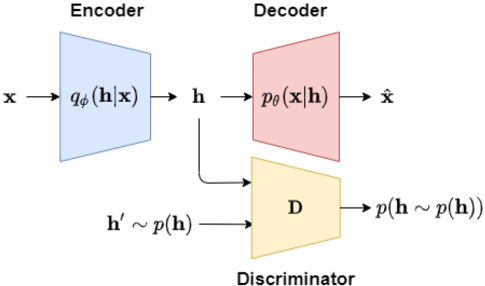
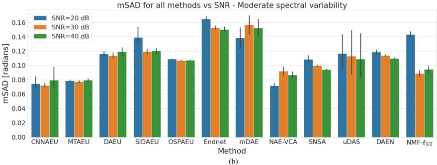
Deep learning (DL) has heavily impacted the data-intensive field of remote sensing. Autoencoders are a type of DL methods that have been found to be powerful for blind hyperspectral unmixing (HU). HU is the process of resolving the measured spectrum of a pixel into a combination of a set of spectral signatures called endmembers and simultaneously determining their fractional abundances in the pixel. This article details the various autoencoder architectures used in HU and provides a critical comparison of some of the existing published blind unmixing methods based on autoencoders. Eleven different autoencoder methods and one traditional method will be compared in blind unmixing experiments using four real datasets and four synthetic datasets with different spectral variability. Additionally, extensive ablation experiments with a simple spectral unmixing autoencoder will be performed. The results are interpreted in terms of the various implementation details, and the question of why autoencoder methods are so powerful compared to traditional methods is unraveled. The source codes for all methods implemented in this article can be found athttps://github.com/burknipalsson/hu_autoencoders.
Overview
The claims and statistics of this paper haven’t been checked yet.
Free: it reads the open-access text and checks the first 5 claims that cite a source we can check. Create a free account to check every claim.
Integrity signals
Registry
Cites
Statistics
Figures






Verification
Claims the paper makes
The claims and statistics of this paper haven’t been checked yet.
Free: it reads the open-access text and checks the first 5 claims that cite a source we can check. Create a free account to check every claim.
Self-check
Percentages, sums and reported differences re-computed from the paper’s own numbers.
The self-check needs the paper’s full text.
Citations
Cites
Hochreiter, S., & Schmidhuber, J. (1997) · Neural Computation · doi:10.1162/neco.1997.9.8.1735 · Cited by 102,318 · cited 1×
“The method in [110] is the first blind HU method to utilize a long short-term memory [111] network.”
Method(2014) · Cited by 33,419
Batch Normalization: Accelerating Deep Network Training by Reducing Internal Covariate Shift
Ioffe, S., & Szegedy, C. (2015) · arXiv · doi:10.48550/arxiv.1502.03167 · Cited by 27,818 · cited 2×
“Batch normalization is used to speed up the training of neural networks and make them more stable through normalization of the inputs to a layer by recentering and rescaling [86].”
BackgroundMethodUnpaired image-to-image translation using cycle-consistent adversarial networks
Zhu, J.-Y., Park, T., Isola, P., & Efros, A. A. (2017) · 2017 IEEE International Conference on Computer Vision (ICCV) · doi:10.1109/iccv.2017.244 · Cited by 23,602
Reducing the dimensionality of data with neural networks
Hinton, G. E., & Salakhutdinov, R. R. (2006) · Science · doi:10.1126/science.1127647 · Cited by 20,928
Auto-Encoding Variational Bayes
Kingma, D. P., & Welling, M. (2013) · arXiv · doi:10.48550/arxiv.1312.6114 · Cited by 20,067
Learning Internal Representations by Error Propagation
Rumelhart, D. E., Hinton, G. E., & Williams, R. J. (1985) · doi:10.21236/ada164453 · Cited by 16,172
(2012) · Cited by 8,009
Practical Bayesian Optimization of Machine Learning Algorithms
Snoek, J., Larochelle, H., & Adams, R. P. (2012) · arXiv · doi:10.48550/arxiv.1206.2944 · Cited by 6,691 · cited 1×
“In recent years, Bayesian optimization [118] has emerged as a state-of-the-art optimization framework for the optimization of blackbox functions, especially expensive ones.”
Background(2017) · International Conference on Machine Learning · Cited by 6,382
Research works printed but not linked: 3
- Goodfellow, 2016, Deep Learning
- Chen, 2015, Marginalized stacked denoising autoencoders, 16, 3849
- Maas, 2013, Rectifier nonlinearities improve neural network acoustic models, 30, 3
Cited by
Autoencoders and their applications in machine learning: a survey
Berahmand, K., Daneshfar, F., Salehi, E. S., Li, Y., & Xu, Y. (2024) · Artificial Intelligence Review · doi:10.1007/s10462-023-10662-6 · Cited by 593
Self-Supervised Learning in Remote Sensing: A review
Wang, Y., Albrecht, C. M., Braham, N. A. A., Mou, L., & Zhu, X. X. (2022) · IEEE Geoscience and Remote Sensing Magazine · doi:10.1109/mgrs.2022.3198244 · Cited by 364
“AUTOENCODERS IN REMOTE SENSING AEs have been widely used to learn representation from various remote sensing data like multispectral images [92]–[99], HSIs [100]–[107], and SAR images [108]–[111].”
MethodHyperspectral Unmixing Using Transformer Network
Ghosh, P., Roy, S. K., Koirala, B., Rasti, B., & Scheunders, P. (2022) · IEEE Transactions on Geoscience and Remote Sensing · doi:10.1109/tgrs.2022.3196057 · Cited by 175
“In [30], autoencoders that have been used for hyperspectral unmixing are grouped into five different categories: (a) Sparse nonnegative autoencoders (a stack of nonnegative sparse autoencoders (SNSA)) [31] (b) Variational autoencoders (Deep AutoEncoder Network (DAEN) [32], Deep Generative Unmixing algorithm (DeepGUn)…”
MethodHyperspectral Unmixing Based on Nonnegative Matrix Factorization: A Comprehensive Review
Feng, X.-R., Li, H.-C., Wang, R., Du, Q., Jia, X., & Plaza, A. (2022) · IEEE Journal of Selected Topics in Applied Earth Observations and Remote Sensing · doi:10.1109/jstars.2022.3175257 · Cited by 178
“Therefore, many researchers have focused on hyperspectral unmixing using autoencoder and its variants, achieving more competitive unmixing performance [41]–[47].”
BackgroundTensor Decompositions for Hyperspectral Data Processing in Remote Sensing: A comprehensive review
Wang, M., Hong, D., Han, Z., Li, J., Yao, J. T., Gao, L., Zhang, B., & Chanussot, J. (2023) · IEEE Geoscience and Remote Sensing Magazine · doi:10.1109/mgrs.2022.3227063 · Cited by 146
“A classic tutorial [244] is presented for practitioners to understand the parallel and distributed computation of big tensors from the perspective of mathematical analytics.”
Background
Metadata
- Authors
- Palsson, B., Sveinsson, J. R., & Ulfarsson, M. O.
- Affiliations
- University of Iceland (IS)
- Venue
- IEEE Journal of Selected Topics in Applied Earth Observations and Remote Sensing
- Published
- 2022
- Volume
- 15
- Pages
- 1340-1372
- ISSN
- 1939-1404 (ISSN-L)
- 2151-1535
- OpenAlex
- W4206620949
- Cited by
- 107
- References
- 132
- Citations by year
- 2026: 16 · 2025: 27 · 2024: 32 · 2023: 24 · 2022: 8
- FWCI
- 8.88
- Type
- journal article
- Language
- en
- Open access
- gold
- doi.org
- Locations
- IEEE Journal of Selected Topics in Applied Earth Observations and Remote Sensing (publishedVersion, cc-by)
- DOAJ (DOAJ: Directory of Open Access Journals) (submittedVersion, cc-by-sa)
- Opin vísindi (Opin vísindi) (submittedVersion, other-oa)
- Opin vísindi (Opin vísindi) (submittedVersion, cc-by-nc-sa)
- Funders
- Icelandic Research Fund (174075-05, 207233-052)
- Topics
- Physical Sciences › Computer Science › Computer Vision and Pattern Recognition › Remote-Sensing Image Classification
- Physical Sciences › Earth and Planetary Sciences › Geochemistry and Petrology › Geochemistry and Geologic Mapping
- Physical Sciences › Chemistry › Analytical Chemistry › Spectroscopy and Chemometric Analyses
- Keywords
- autoencoder, endmember extraction, fractional abundance estimation, spectral signatures, ablation study, deep learning for remote sensing
About these checks
Registry, retraction, Cites and statistics results are computed, not judged, with one exception: a printed reference that no index lists is read once by a model before it counts as a citation error. Claims are extracted by a model and kept only when their quote appears verbatim in the text; each cited source is then checked, with a model’s help, for whether it says what the claim relies on. Those verdicts can be wrong — read the claim’s quote and the cited source before relying on one.
Statistics and arithmetic are recomputed, not judged.
Confidence bands are shown only for fields calibrated on our annotated test set. None is calibrated yet, so no band is shown.
What counts as a claim ›How we measure confidence ›How we check this ›
Are you an author, or do you see a problem with this page? Request a review
How to cite
Cite CoChat for the checks on this page, and the paper for its own findings.
- This page
- CoChat. (2026). Citation check: Blind Hyperspectral Unmixing Using Autoencoders: A Critical Comparison. https://app.cochat.ai/papers/10.1109/jstars.2021.3140154
- The paper
- Palsson, B., Sveinsson, J. R., & Ulfarsson, M. O. (2022). Blind Hyperspectral Unmixing Using Autoencoders: A Critical Comparison. IEEE Journal of Selected Topics in Applied Earth Observations and Remote Sensing. https://doi.org/10.1109/jstars.2021.3140154
Data sources
Bibliographic data: Semantic Scholar, OpenAlex, Crossref.
Contains information from the Semantic Scholar Academic Graph Datasets, made available under the ODC Attribution License (ODC-BY 1.0).
Semantic Scholar’s data is described in: Kinney, R., et al. (2023). The Semantic Scholar Open Data Platform. arXiv:2301.10140.
